Dashboard Apps
The Kāhu dashboard apps allow you to monitor and calibrate the system, and run simple NMR and MRI experiments with just a few button clicks.
To find the dashboard apps, click the waveform icon in the JupyterLab interface’s left panel.
App Tools and Features
Most of the apps share common tools and features, and it is useful to familiarise yourself with these common features before you begin exploring each app.
Running Apps
Most dashboards have a control bar with the following features.
Run - Click the green “Run” button to run a dashboard. This button will grey out while the dashboard is running. While a dashboard is running, all other dashboards will be disabled.
Abort - Click the red “Abort” button to stop a dashboard that is running.
Progress Bar - This bar shows the estimated progress in green.
Status Bar - This bar will display the dashboard’s current status and error messages.
Common status messages are:
Running - The dashboard is currently running, even if there is not visible progression on the progress bar.
Finished - The dashboard has completed its process.
Busy - The dashboard is unable to run because Kāhu is already running a pulse sequence. Either find the dashboard that is currently running a sequence and click the Abort button, or use Admin:System Reset in the System dashboard to stop any sequence that is running.
Saving Data
Data from the dashboard apps can be saved using the save options located beneath the control bar.
Saving directory - will save the data to “user/data/<Workspace>/<File Name>”. Subdirectories can also be specified using a “/”, e.g. “kerry/3D” to save to “user/data/kerry/3D/<File Name>”.
File name - will save with this file name within the chosen workspace directory, as in the image below.
Save - save the data (data will not be autosaved).
When you save data from the dasboard apps, two files will be saved. The first file is a “.npy” file which contains the k-space data from the experiment and the second file is a “.yaml” file which contains the pulse sequence parameters that were used in the experiment.
Autosaved Parameters
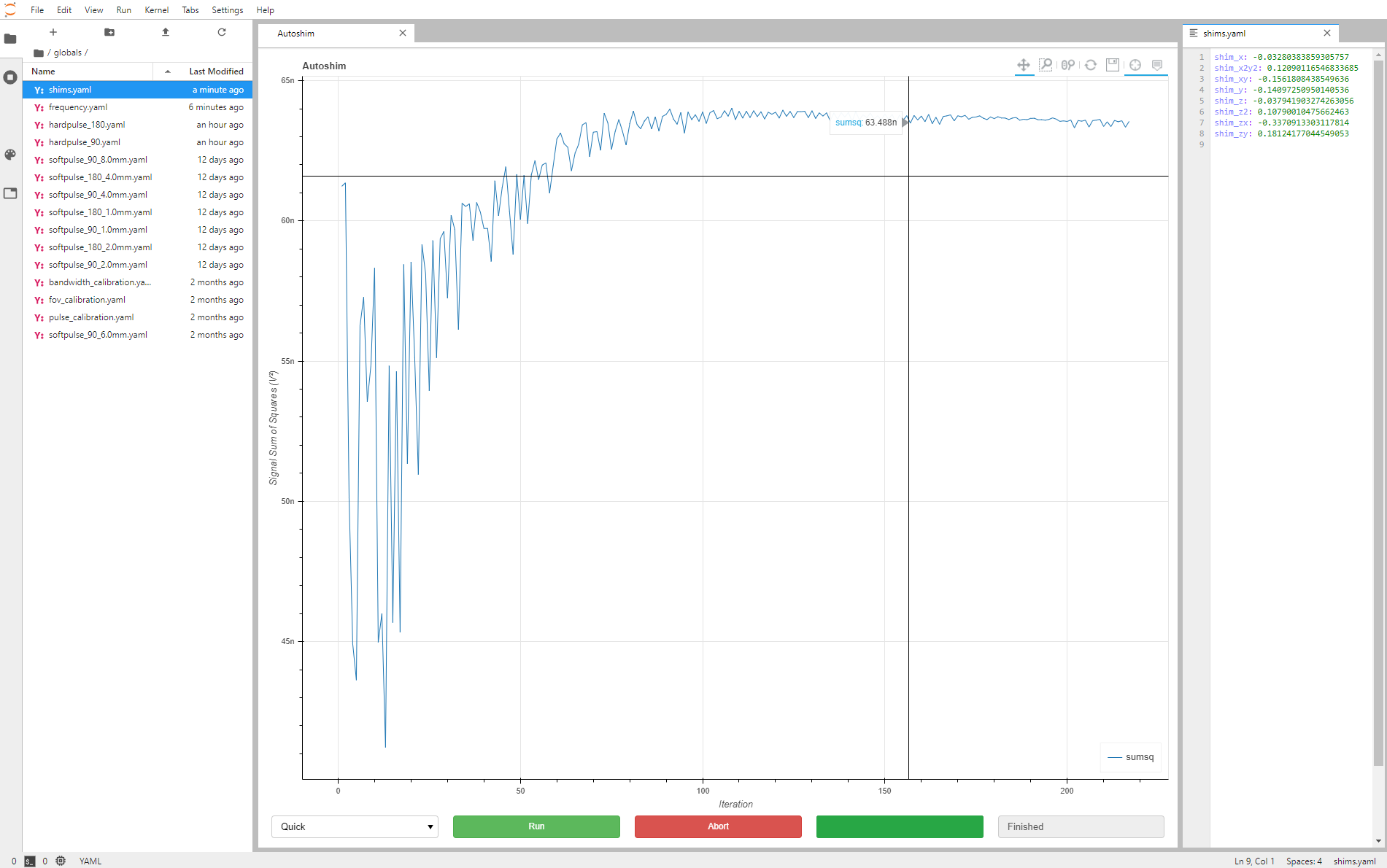
The dashboard apps used for configuring and setting up the instrument will automatically update system parameters when run. These system parameter sets can be found in files in the “globals” directory as shown in the image below. These files are not intended to be changed manually under normal circumstances.
General
System
Temperature Monitor
The first step in the Kāhu setup process is to check the Temperature dashboard. The magnet in Kāhu is temperature controlled to keep the system frequency stable and uses a PT100 sensor to measure its temperature. The sensor results are this displayed on the dashboard.
Note
The set control point is 30°C, please ensure that the system has reached and held 30°C for at least 30 minutes before continuing with the setup process.
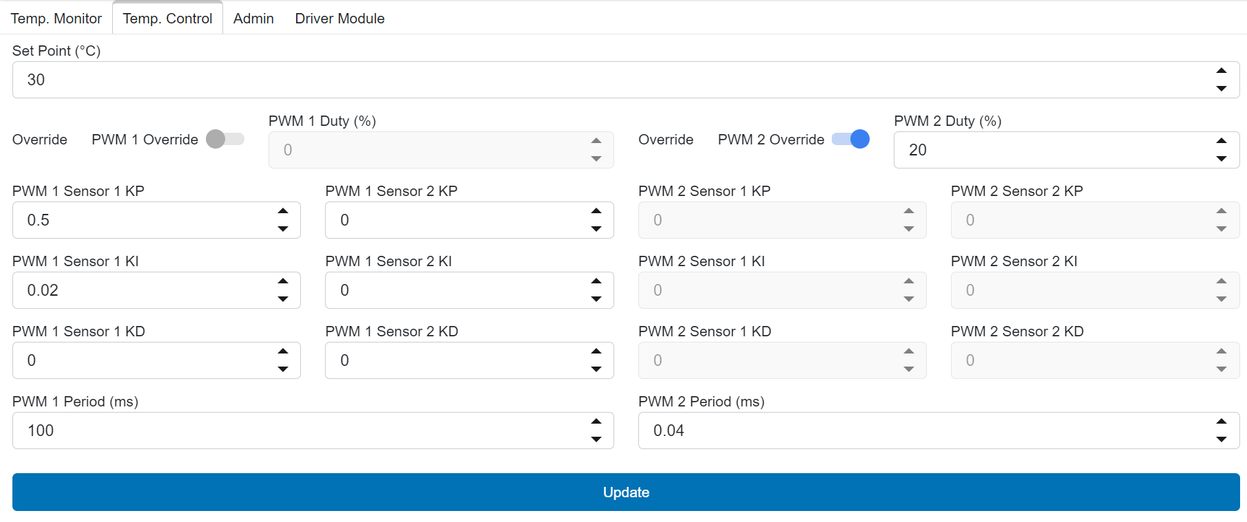
Temperature Control
Attention
Please use the recommended default values for KP, KI, and KD. The Set Point may be adjusted when operating in warm or cold environments. It is recommended to use a set point 5°C above room temperature if 30°C is not stable.
The recommended default values are:
Admin
This dashboard is not part of the setup process but is important to take note of as it controls two key functions: Resetting the Driver and Shutting Down the System
- System Reset:
This will abort any sequence that is currently running and reset Kāhu to standby state, ready to run sequences.
- System Shutdown:
When you want to shut down the system, toggle the “Enable” switch and click “Shutdown”.
Attention
To avoid data loss, please always use the admin dashboard when you need to shutdown Kāhu.
Driver Module
Allows setting the gain of the RF Amp module receive amplifier. A value of 21 dB is recommended.
Utilities
When you first set up your Kāhu, it is important to run through the utility apps. This will ensure that your system has been properly prepared before you begin your magnetic resonance experiments.
Find Frequency
Runs a pulse collect acquisition with a short, full power pulse. The frequency will be automatically calculated from the peak in the spectrum and saved to the globals/frequency.yaml file every time this app is run.
- When initially finding the NMR frequency on first setup:
Edit the globals/frequency.yaml file with an estimate of your NMR frequency calculated from field strength and gyromagnetic ratio
set a short dwell-time (t_dw) of 0.2µs to achieve a large bandwidth and increase the apodization to 10,000 Hz to reduce noise. Increase the number of scans if SNR is low.
If the probe has a high Q, try retuning to different values around the expected NMR frequency as it will not be sensitive to NMR frequencies outside its small bandwidth.
- Once the NMR frequency has been found and the probe tuned:
Increase t_dw to acquire for a longer duration.
Decrease apodization to an appropriate level for the natural linewidth of the FID (e.g. 10 Hz)
This will increase the precision of the calculated frequency value.
Noise Check
Runs an acquisition on all channels and plots the signal and spectrum of the noise.
Run Loop may be used to monitor the noise continuously. Click Abort to stop before attempting to run other experiments.
Tune Match
Transmits a frequency sweep of the given bandwidth centred on the global frequency on all Tx channels while acquiring on all Rx channels. The y-axis of reflected signal plot is in dB relative to the largest value present.
Run Loop may be used to monitor the reflected signal continuously while tuning/matching a probe. Click Abort to stop before attempting to run other experiments.
Pulse Calibration
Steps through all amplitude values and plots the resulting signal intensity. Automatically calculates the 90 and 180 pulse amplitudes from the first maximum and subsequent minimum and saves the calibrated pulses to globals/hardpulse_90.yaml and globals/hardpulse_180.yaml.
Ensure the t_end repetition delay is long enough to avoid T1 effects from the sample.
Autoshim
Optimises the shim settings iteratively to maximise the sum of squares of the apodized FID. The shim values should converge and flatten out.
Note: The apodization is not applied to the plotted signal, only to the signal used for optimisation.
ilumr
These applications are a port of those used in the ilumr desktop MRI system, using a compatibility mode that assumes:
Tx 0 is used for transmit
Rx 0 is used for receive
Pin 1 of GPO 0 is used to control the T/R switch
With the Kāhu 0.3T MRI System, follow the Hardware Setup guide to ensure the hardware is set up correctly.
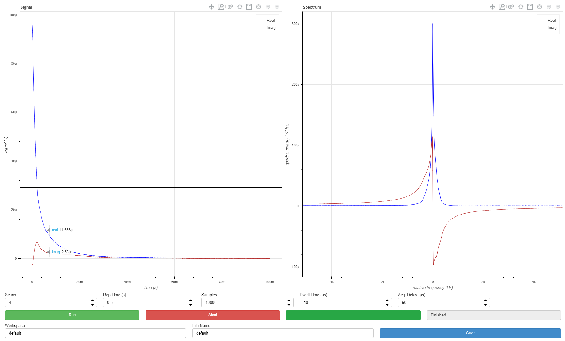
FID
This experiment runs a Free Induction Decay pulse sequence with the following parameters:
Scans - can be used to improve the signal-to-noise ratio (SNR) by averaging multiple scans.
Rep Time - time waited between scans, may need to be increased for samples with a long T1 recovery time (e.g. pure water).
Samples - number of complex samples acquired.
Dwell Time - time between sample, longer dwell time will result in a narrower bandwidth in the Spectrum plot on the right.
Acq. Delay - time delay after the RF pulse to allow for probe/duplexer dead time, should not need to be modified.
Note
Frequency, pulse power/width, and shim settings are read from the global system parameter files every time the experiment is run, and cannot be set manually in the dashboard.
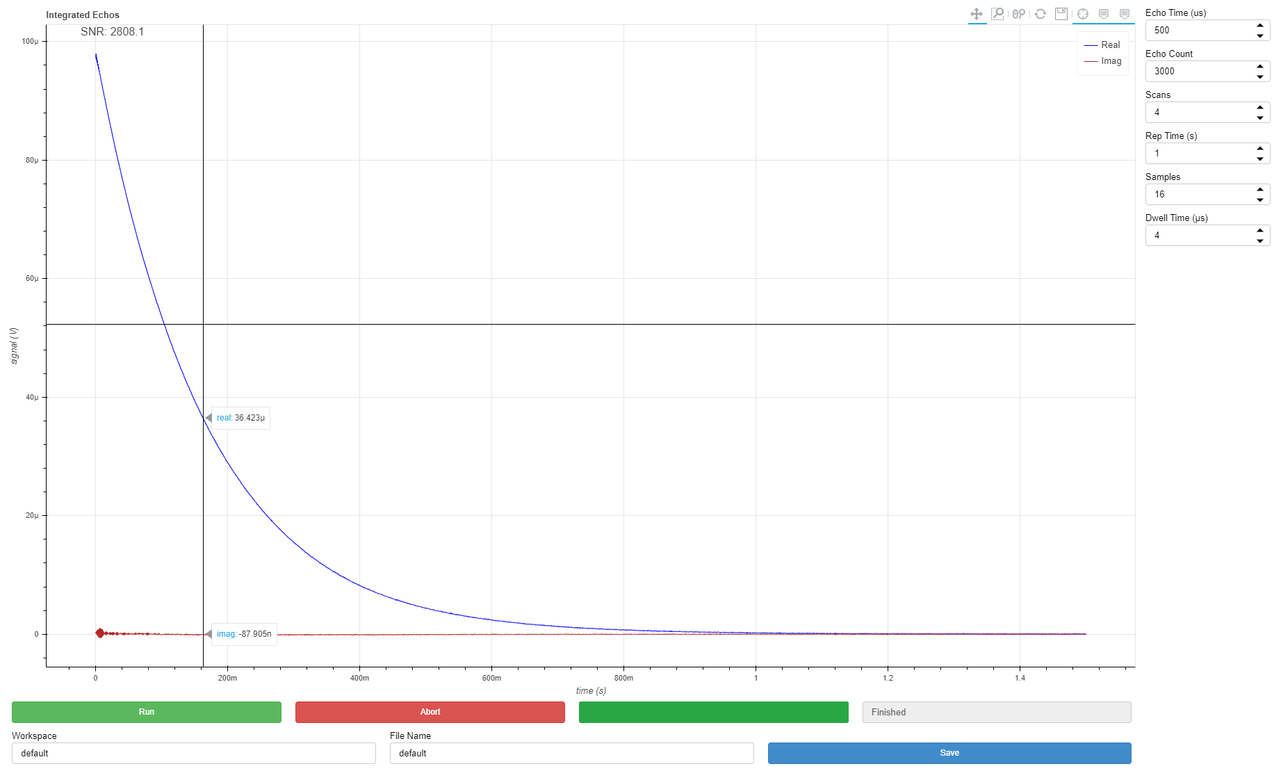
CPMG
This experiment runs a Carr-Purcell-Meiboom-Gill pulse sequence, repeated “Scans” times with 2 or 4 step phase cycling with the following parameters:
Scans - can be used to improve the signal-to-noise ratio (SNR) by averaging multiple scans. Use 2 or a multiple of 4 scans for best results.
Rep Time - time waited between scans, may need to be increased for samples with a long T1 recovery time (e.g. pure water).
Samples - number of complex samples acquired per echo.
Dwell Time - time between samples.
Echo Time - time between 180 degree RF pulses, determines the time between data point on the Integrated Echos plot.
Echo Count - number of echos, determines number of points on the Integrated Echos plot.
Note
Frequency and pulse power/width are read from the global system parameter files every time the experiment is run, and cannot be set manually in the dashboard.
1D SE
This experiment runs a Spin Echo pulse sequence with a frequency encoding gradient for 1D projection imaging, and optionally using soft 90 pulse with slice gradient for slice selection (can be applied along the same direction as the frequency encode gradient to measure the slice profile). Parameters:
Scans - can be used to improve the signal-to-noise ratio (SNR) by averaging multiple scans.
Rep Time - time waited between scans, may need to be increased for samples with a long T1 recovery time (e.g. pure water).
Freq Enc Res - desired spatial resolution of the image along the frequency encode axis.
Freq Enc Axis - selects which gradient to use for frequency encoding, or no gradient if N.
Slice Width - desired spatial width of the slice.
Slice Offset - desired spatial offset of slice along the slice axis.
Slice Axis - selects which gradient to use for slicing, or no gradient if N. The experiment will use a hard 90 pulse when this option is set to N.
The following post processing parameters are for smoothing and scaling the data:
Gaussian Blur - windows the data prior to Fourier reconstruction to filter out high frequency artefacts and increase SNR at the expense of resolution. Use 0 for no blurring.
Upscaling - zero fills the data prior to Fourier reconstruction to reduce pixellation and give a smoother image. Use 1 for no upscaling.
Note
Frequency, pulse power/width, and shim settings are read from the global system parameter files every time the experiment is run, and cannot be set manually in the dashboard.
2D RARE
This experiment runs a RARE pulse sequence with optional slicing, frequency encode, and phase encode for either 2D projection or 2D slice imaging parameters:
Scans - can be used to improve the signal-to-noise ratio (SNR) by averaging multiple scans.
Rep Time - time waited between scans, may need to be increased for samples with a long T1 recovery time (e.g. pure water).
Freq Enc Res - desired spatial resolution of the image along the frequency encode axis.
Freq Enc Axis - selects which gradient to use for frequency encoding, or no gradient if N.
Phase Enc Res - desired spatial resolution of the image along the phase encode axis.
Phase Enc Axis - selects which gradient to use for phase encoding, or no gradient if N.
Slice Width - desired spatial width of the slice.
Slice Offset - not supported at time of writing, for more information please contact Resonint.
Slice Axis - selects which gradient to use for slicing, or no gradient if N. The experiment will use a hard 90 pulse when this option is set to N.
The following post processing parameters are for smoothing and scaling the data:
Gaussian Blur - windows the data prior to Fourier reconstruction to filter out high frequency artefacts and increase SNR at the expense of resolution. Use 0 for no blurring.
Upscaling - zero fills the data prior to Fourier reconstruction to reduce pixellation and give a smoother image. Use 1 for no upscaling.
Note
Frequency, pulse power/width, and shim settings are read from the global system parameter files every time the experiment is run, and cannot be set manually in the dashboard.
2D RARE Advanced
The 2D RARE advanced dashboard is an expansion of the standard 2D RARE dashboard. The additional controllable parameters make it better suited for contrast imaging experiments. .. and list other things it is more useful for
As well as the standard 2D RARE parameters, 2D RARE Advanced includes the following parameters:
Echo Train Length (ETL)
Effective Echo Time (TE_eff)
3D RARE
This experiment runs a RARE pulse sequence with frequency encode along one axis and phase encode along two axes. The number of echos in the CPMG sequence is set by Phase Enc 2 Res and the whole CPMG sequence is repeated Phase Enc 1 Res times, with appropriate phase gradient pulses.
Parameters:
Scans - can be used to improve the signal-to-noise ratio (SNR) by averaging multiple scans.
Rep Time - time waited between scans, may need to be increased for samples with a long T1 recovery time (e.g. pure water).
Freq Enc Res - desired spatial resolution of the image along the frequency encode axis.
Freq Enc Axis - selects which gradient to use for frequency encoding, or no gradient if N.
Phase Enc 1 Res - selects which gradient to use for the first phase encoding, or no gradient if N.
Phase Enc 1 Axis - selects which gradient to use for phase encoding, or no gradient if N.
Phase Enc 2 Res - desired spatial resolution of the image along the second phase encode axis.
Phase Enc 2 Axis - selects which gradient to use for the second phase encoding, or no gradient if N.
The following post processing parameters are for smoothing, scaling, and viewing the data:
Gaussian Blur - windows the data prior to Fourier reconstruction to filter out high frequency artefacts and increase SNR at the expense of resolution. Use 0 for no blurring.
Upscaling - zero fills the data prior to Fourier reconstruction to reduce pixellation and give a smoother image. Use 1 for no upscaling.
View Slice index - set the slice axis with the F/P1/P2 radio buttons (physical axis will depend on above settings) and drag the View Slice Index slider to move the slice plane through the 3D data.
Note
Frequency, pulse power/width, and shim settings are read from the global system parameter files every time the experiment is run, and cannot be set manually in the dashboard.
3D FISP
This experiment runs a FISP (also called GRASS) pulse sequence with frequency encode along one axis and phase encode along two axes. Parameters:
Scans - can be used to improve the signal-to-noise ratio (SNR) by averaging multiple scans.
TR - time between RF pulses; affects T1 contrast and pulse sequence duration.
Flip Angle - sets the flip angle of the RF pulse used.
Freq Enc Res - desired spatial resolution of the image along the frequency encode axis.
Freq Enc Axis - selects which gradient to use for frequency encoding, or no gradient if N.
Phase Enc 1 Res - desired spatial resolution of the image along the first phase encode axis.
Phase Enc 1 Axis - selects which gradient to use for the first phase encoding, or no gradient if N.
Phase Enc 2 Res - desired spatial resolution of the image along the second phase encode axis.
Phase Enc 2 Axis - selects which gradient to use for the second phase encoding, or no gradient if N.
The following post processing parameters are for smoothing, scaling, and viewing the data:
Gaussian Blur - windows the data prior to Fourier reconstruction to filter out high frequency artefacts and increase SNR at the expense of resolution. Use 0 for no blurring.
Upscaling - zero fills the data prior to Fourier reconstruction to reduce pixellation and give a smoother image. Use 1 for no upscaling.
View Slice index - set the slice axis with the F/P1/P2 radio buttons (physical axis will depend on above settings) and drag the View Slice Index slider to move the slice plane through the 3D data.
Note
Frequency, pulse power/width, and shim settings are read from the global system parameter files every time the experiment is run, and cannot be set manually in the dashboard.
Slice Viewer
Data saved from 3D RARE or 3D FISP experiments can be loaded to view in the slice viewer. Specify Workspace and Filename as when saving and click Load.
The following post processing parameters are for smoothing, scaling, and viewing the data:
- Gaussian Blur - windows the data prior to Fourier reconstruction to filter out high
frequency artefacts and increase SNR at the expense of resolution. Use 0 for no blurring.
- Upscaling - zero fills the data prior to Fourier reconstruction to reduce pixellation and
give a smoother image. Use 1 for no upscaling.
- View Slice index - set the slice axis with the X/Y/Z radio buttons (physical axis will
depend on experiment settings) and drag the View Slice Index slider to move the slice plane through the 3D data.
Noise Check
Once the system temperature is stable, you can perform a Noise Check. This dashboard allows you to assess whether the operating environment is suitable for Kāhu with no large sources of electrical interference. When you run this dashbaord the system will measure and display the environmental noise level.
Click “Run” for a single measurement or “Run Loop” for continuous measurements.
Interference will show up as large spikes extending higher then the baseline noise level. The RMS of the noise signal is displayed in the top left, and should be less than 0.3 µV when using a dwell time of 1 µs.
Note
Note that the data shown here is raw data from the hardware decimator, which does not have a flat frequency response, so the noise spectrum (right-hand plot) will normally have a bell-curve-like shape as shown below.
Find Frequency
The next dashboard to run is Find Frequency which uses an free induction decay (FID) pulse sequence with several dwell time increments in order to determine the NMR frequency of the magnet.
Begin by setting up the sample grip with a collar and shim sample as shown.
Center the provided shim sample with the window in the depth gauge and then insert into the magnet.
Press “Run” to perform the experiment and determine the NMR frequency. The new frequency value is automatically saved and can be found in the following location:
globals/frequency.yaml
Tune Match
The RF probes supplied with Kāhu have been tuned to the magnet’s resonant frequency. However, due to differences in operating environments, this frequency may shift slightly. It is important to have the probe tuned to the current magnet frequency, so before running NMR experiments use the Wobble dashboard to check and adjust the probe tuning if required.
In the graph below, the dotted line indicates the magnet frequency, taken from the frequency found in the previous dashboard. This is an example of a well tuned probe, small offsets from the NMR frequency are not a problem and may also be caused by a change in sample. Try removing the shim sample while running the wobble in looped mode to see the effect.
A well tuned probe should meet the following requirements:
Tune: NMR frequency +/- 0.02MHz
Match: less then 20 µV (20e-6) at NMR frequency
If the probe tunings falls outside of these requirements then please follow the next steps:
Click “Run Loop” on the Wobble dashboard.
Remove the top disk by rotating anti-clockwise
Identify the tune and match capacitors using the provided image. The bottom tune/match capacitor is for coarse adjustment and the top for fine adjustment.
Identify the alignment arrows and notches on the capacitors. Each capacitor has a tiny arrow on the turning part and a notch on the rim. One end of the adjustment range is reached when the arrow is aligned with the notch, and the other end is reached when the arrow is pointing in the opposite direction.
Use the supplied trimmer too to adjust the fine capacitors to 90° from the notch (the halfway point of its range).
Adjust the coarse capacitors to get the tune/match roughly correct.
Then use the fine capacitors to refine the tune/match.
Note
Note that the presence of the trimmer tool will shift the value so remove after each small adjustment to check.
Pulse Calibration
Once the tuning/matching of the probe has been confirmed, the pulse power of 90 and 180 degree RF pulses can be calibrated using the Pulse Calibration dashboard.
The default settings should be adequate when using the 11 mm RF probe (provided as default with Kāhu), but the 15 mm RF probe will require a longer Pulse Width (recommended 60 us) and a greater Number of Steps (recommended 100) to achieve a 180 degree tipping angle.
Once pulse calibration is complete, vertical dotted lines will show the amplitudes of the 90 and 180 degree pulses and the settings will be automatically save to the following files (when not calibrating a soft pulse):
globals/hardpulse_90.yaml
globals/hardpulse_180.yaml
To calibrate soft pulses for MRI slice experiments, check the Soft Pulse option and set the desired Slice Width. The pulse width will auto-populate with a value that should be suitable. When calibration is finished, the settings will be saved to files named:
globals/softpulse_90_<slice width>mm.yaml
globals/softpulse_180_<slice width>mm.yaml
If the 180 degree tipping angle is not reached, the corresponding file will not be created.
Autoshim
The final setup step is determining the electrical shim settings, which is done by Autoshim. The first time this is run after power up (and leaving for some time for the temperature to stabilise) the Coarse setting should be selected in the bottom left for it to start from scratch. A Quick shim can be run periodically to re-optimise the homogeneity if it has drifted (due to small changing thermal gradients in the magnet). The shim values are automatically saved to the shims file (with values in the range [-1, 1]):
globals/shims.yaml