Kāhu 0.3T Desktop MRI

Hardware Setup

This section will guide you through the setup process for the 0.3T Kāhu configuration.

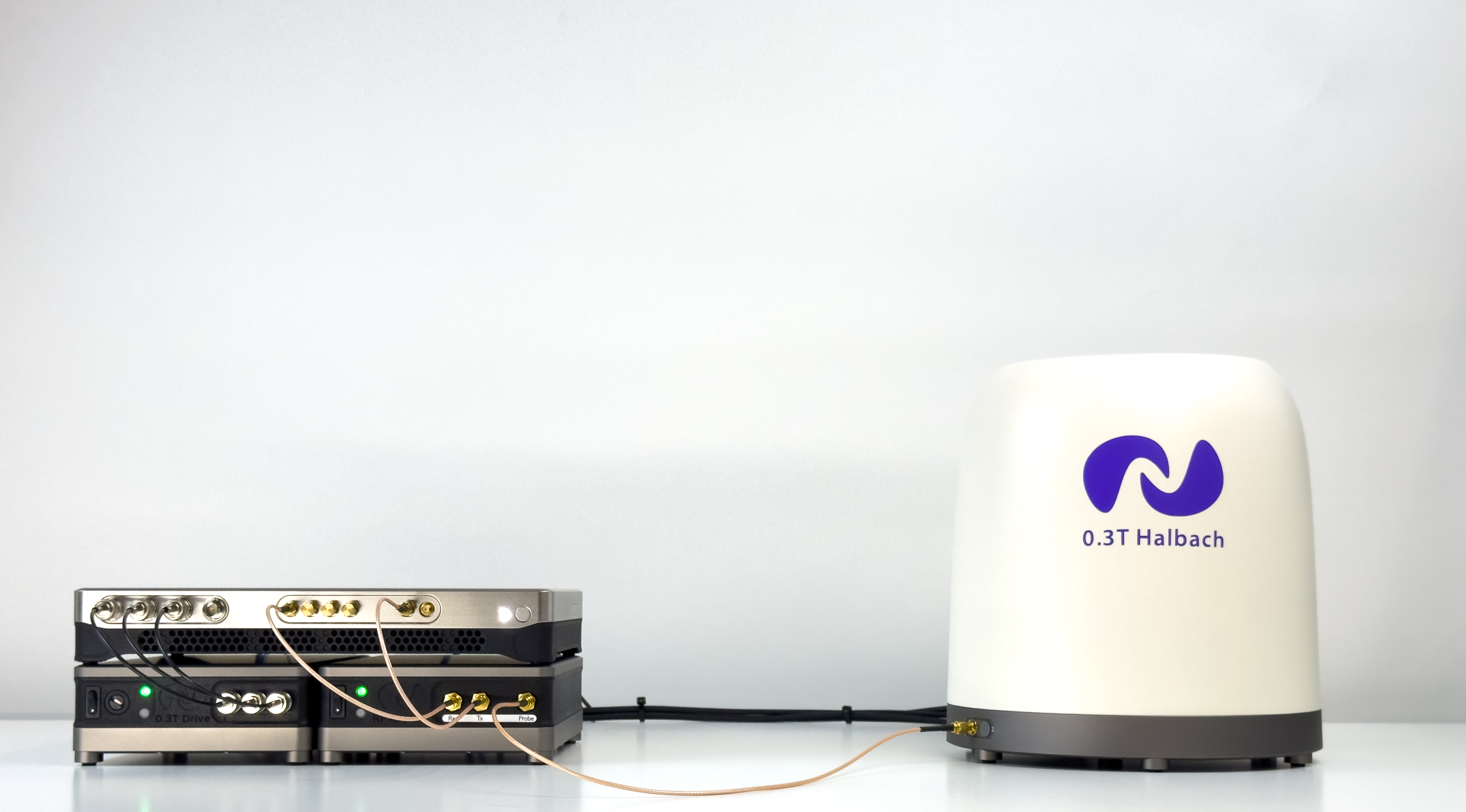
The configuration consists of a Kāhu Spectrometer and the following components:

5W RF Amplifier

This module contains:

• RF power amplifier for transmit

• Transmit/Receive switch

• RF preamplifier for receive

• Removable quarter wave line

0.3T Drive

This module contains:

• 3 Gradient amplifier channels

• 5 Shim amplifier channels

• 1 Heater driver controlled by Temp. Control PWM 1

• 1 Fan driver controlled by Temp. Control PWM 2

0.3T Magnet

This module contains:

• 0.3T Magnet

• Gradient & Shim coils

• Magnet Heater and PT100 Temperature Sensor

• Removeable RF Probe

Note

Please follow these steps carefully before powering up Kāhu and the Drive Modules.

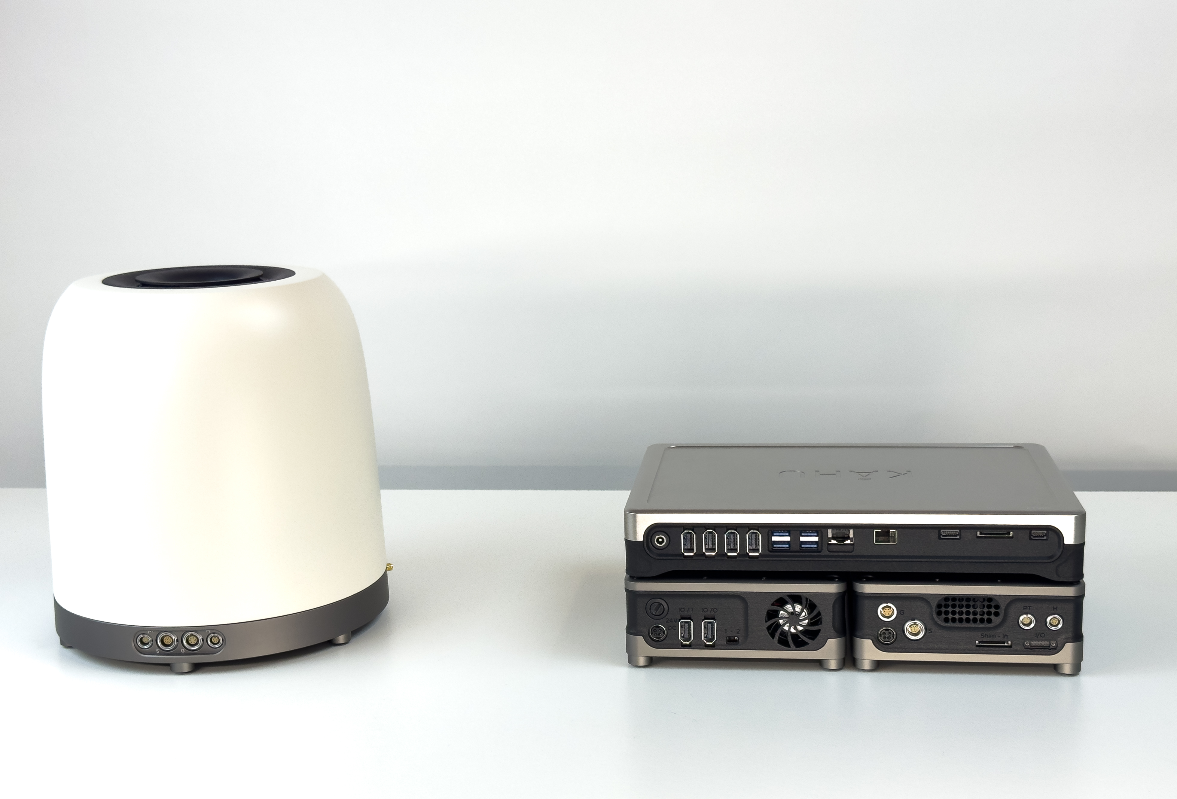
Step 1 - Rear cable connections

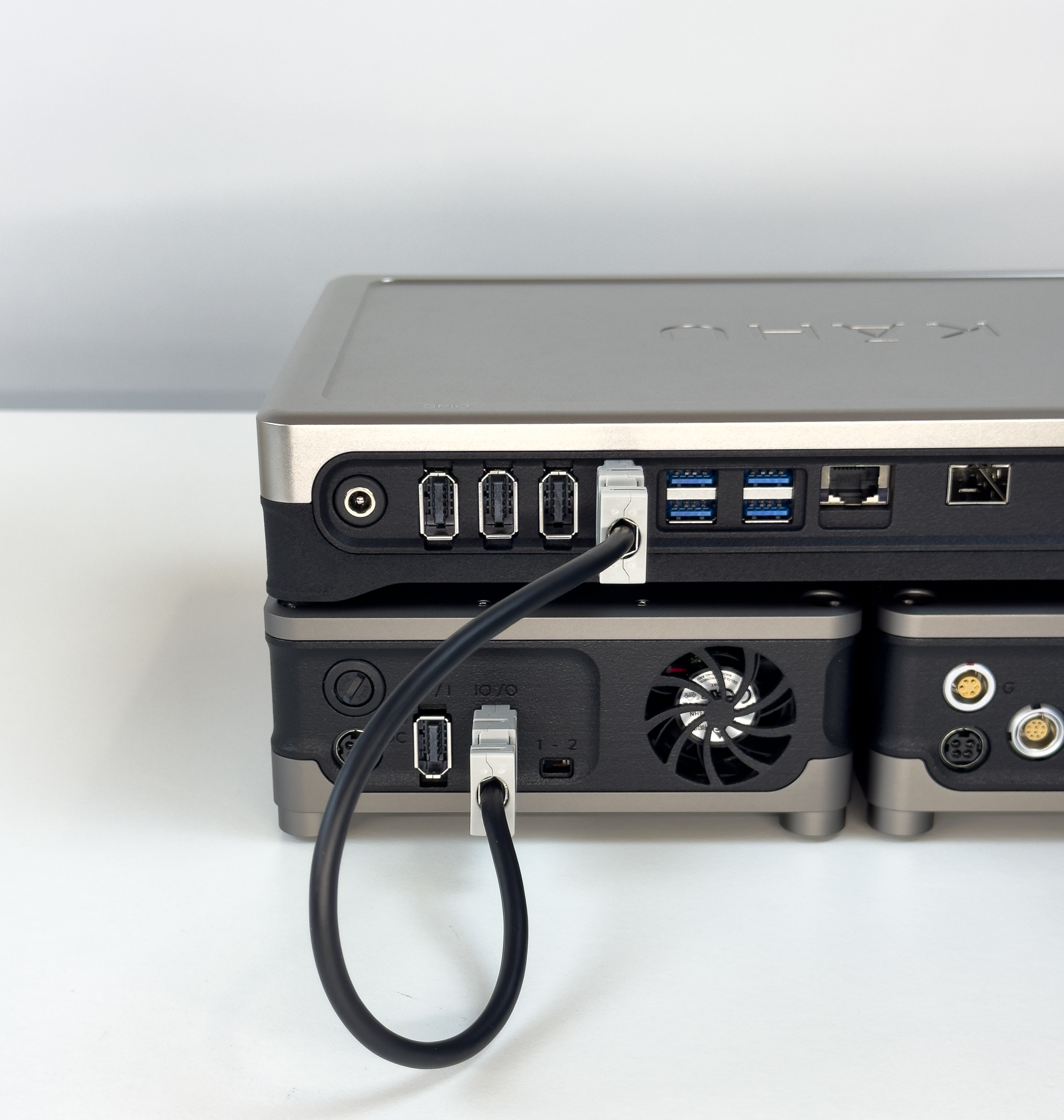
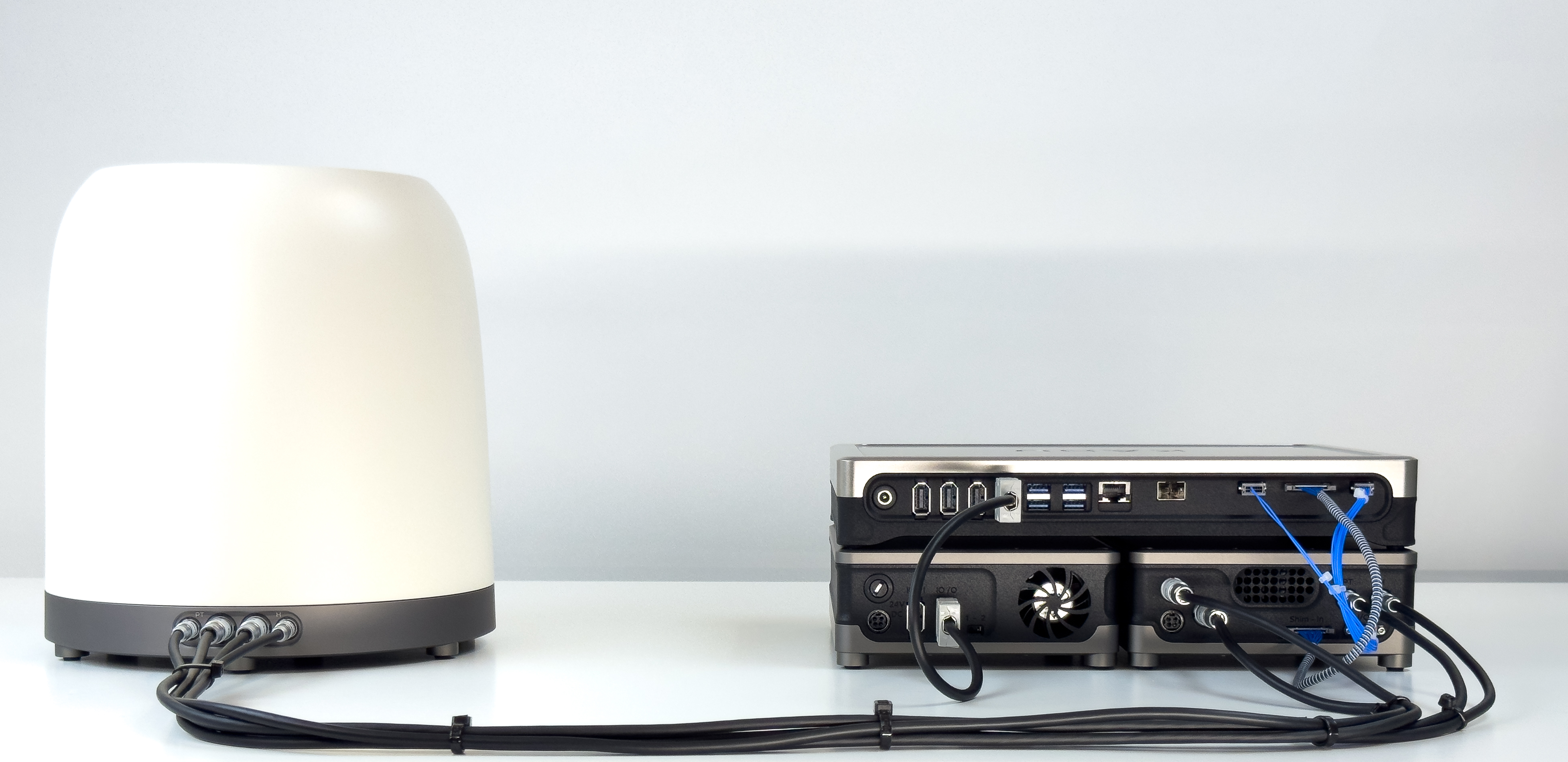
Begin by arranging the modules as shown in the image below with the Kahu Spectrometer placed on top of the drive modules. When viewed from the back, the RF Amplifier is placed on the left and the 0.3T Drive module is placed on the right.

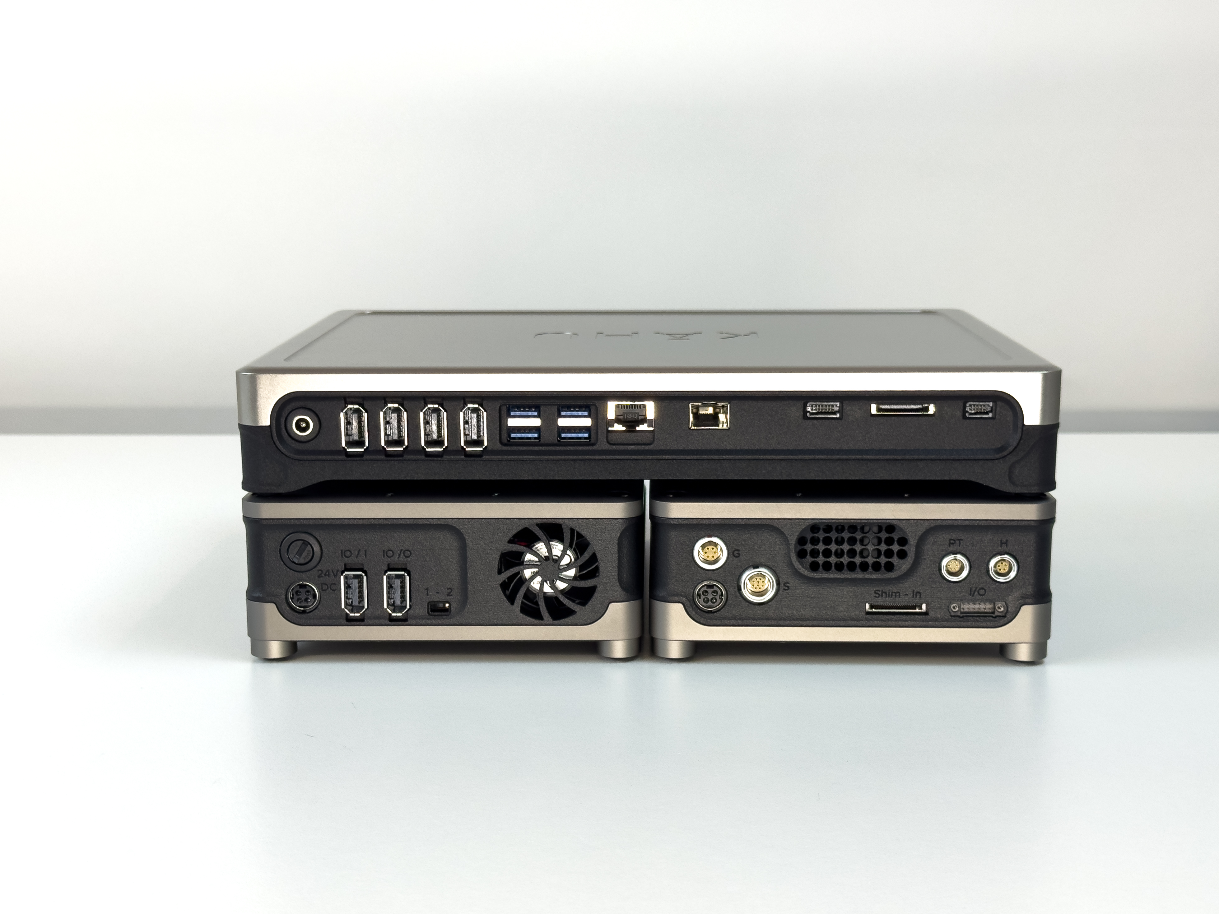
Place the magnet assembly to the left of the drive hardware (when viewed from the back).

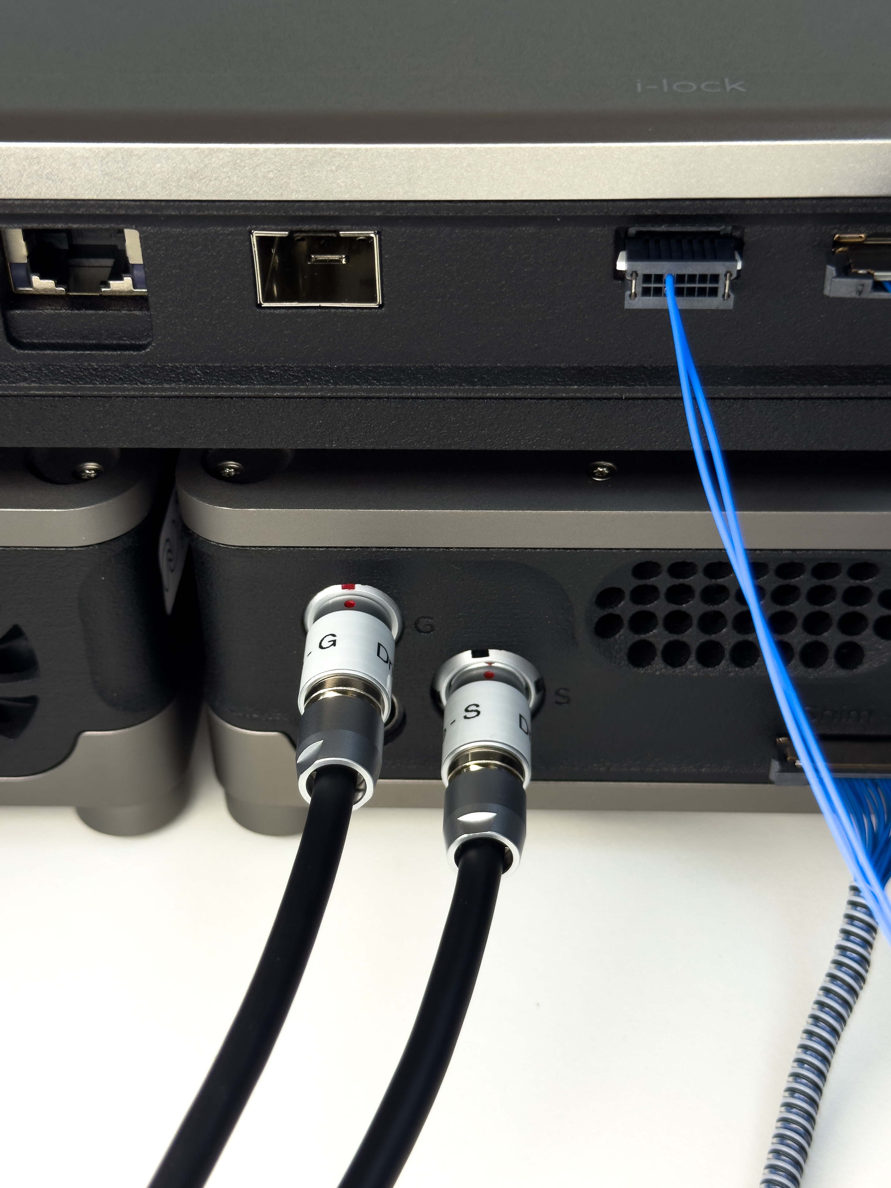
Connect the Kahu i-lock and PT100 ports to the drive module as shown, fastening the I/O connector with the drive tool. Take care to not overtighten.

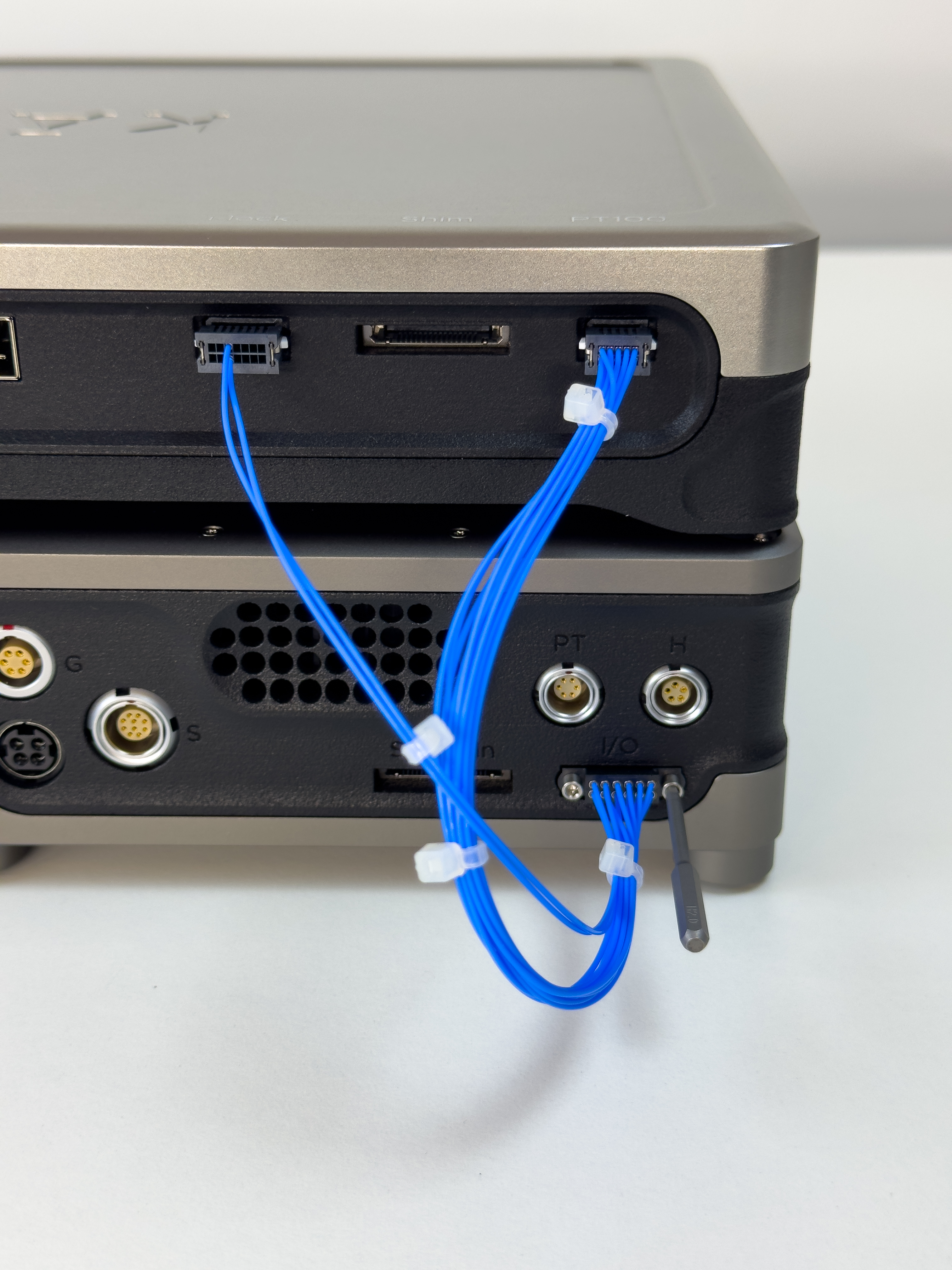
Connect the Shim control cable, note that the cable is oriented with the gold contacts on top for the connection to the Kahu spectrometer.

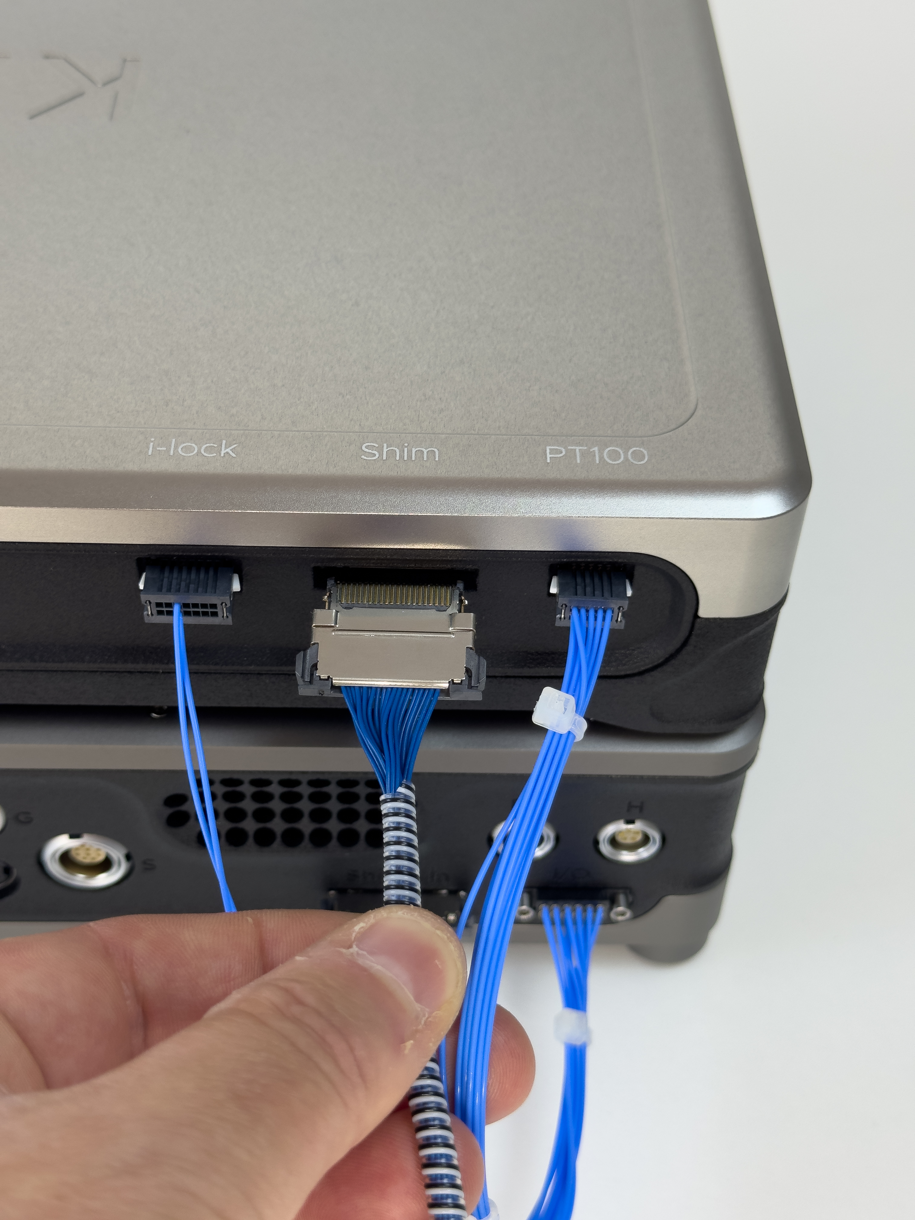
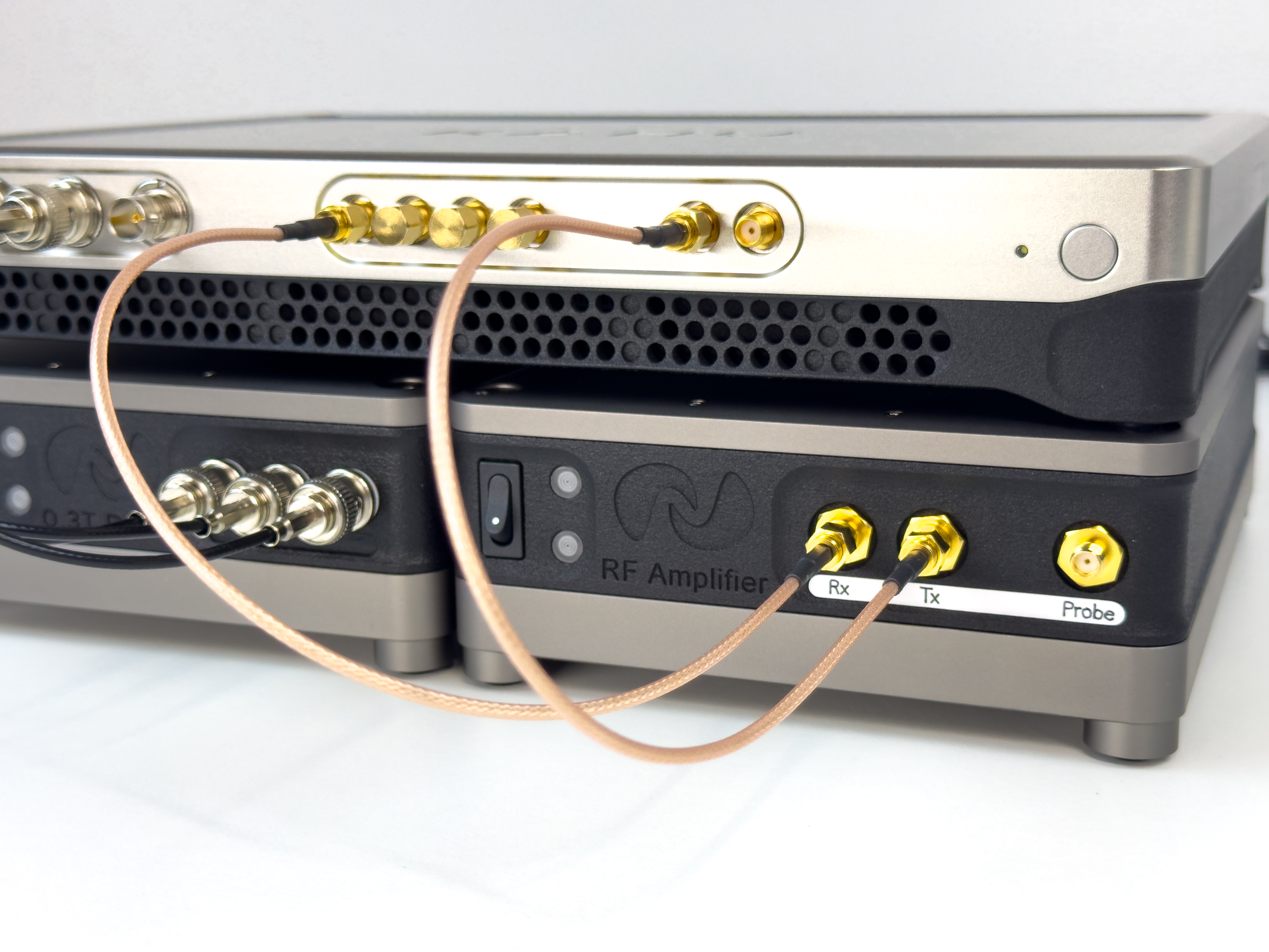
Connect I/O port 0 of the Kāhu Spectrometer to port O of the RF amplifier as shown.

Connect the Drive Module cable loom to the magnet.

Attention

Take care to follow the connector markings to avoid damage!

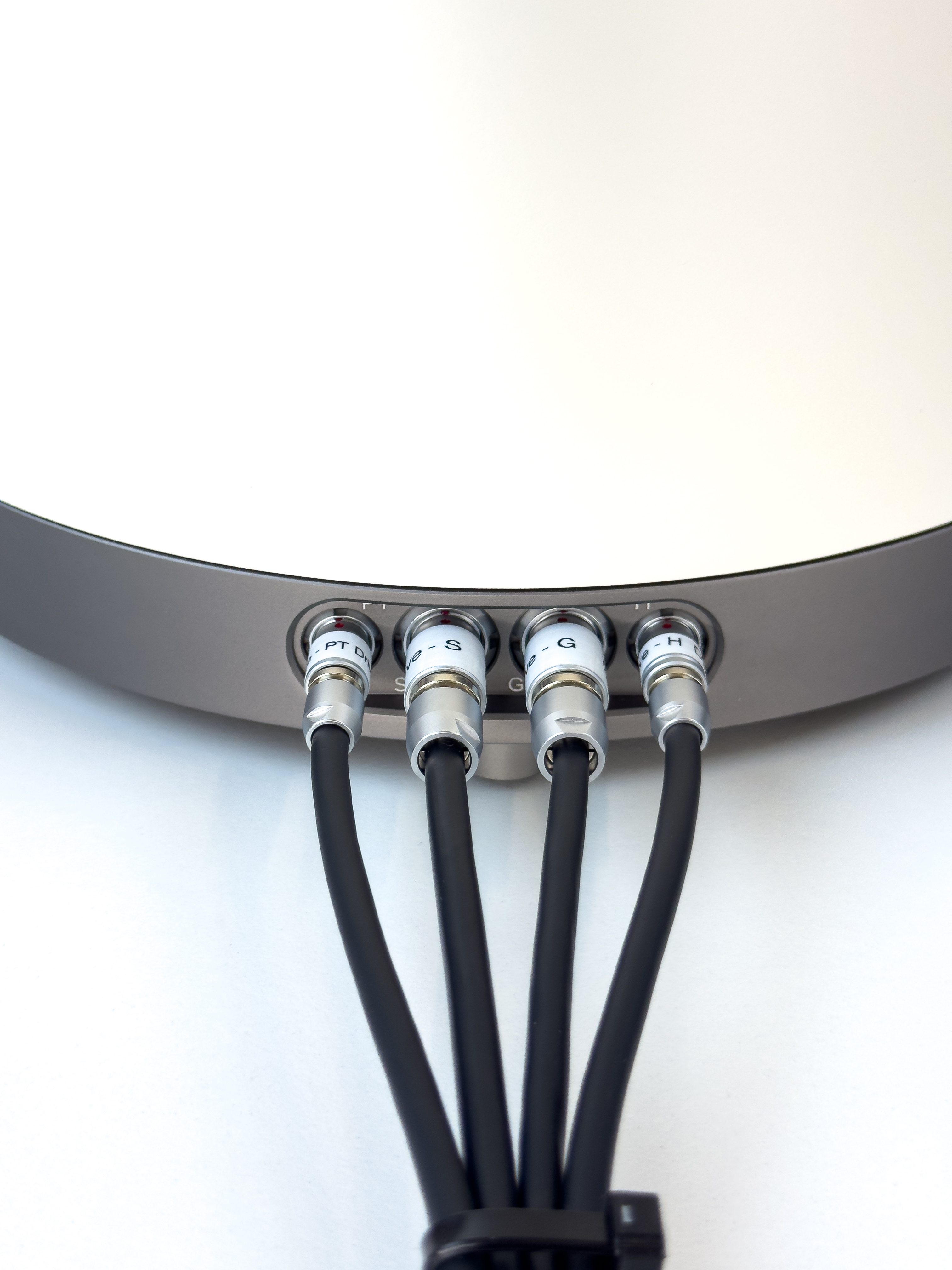
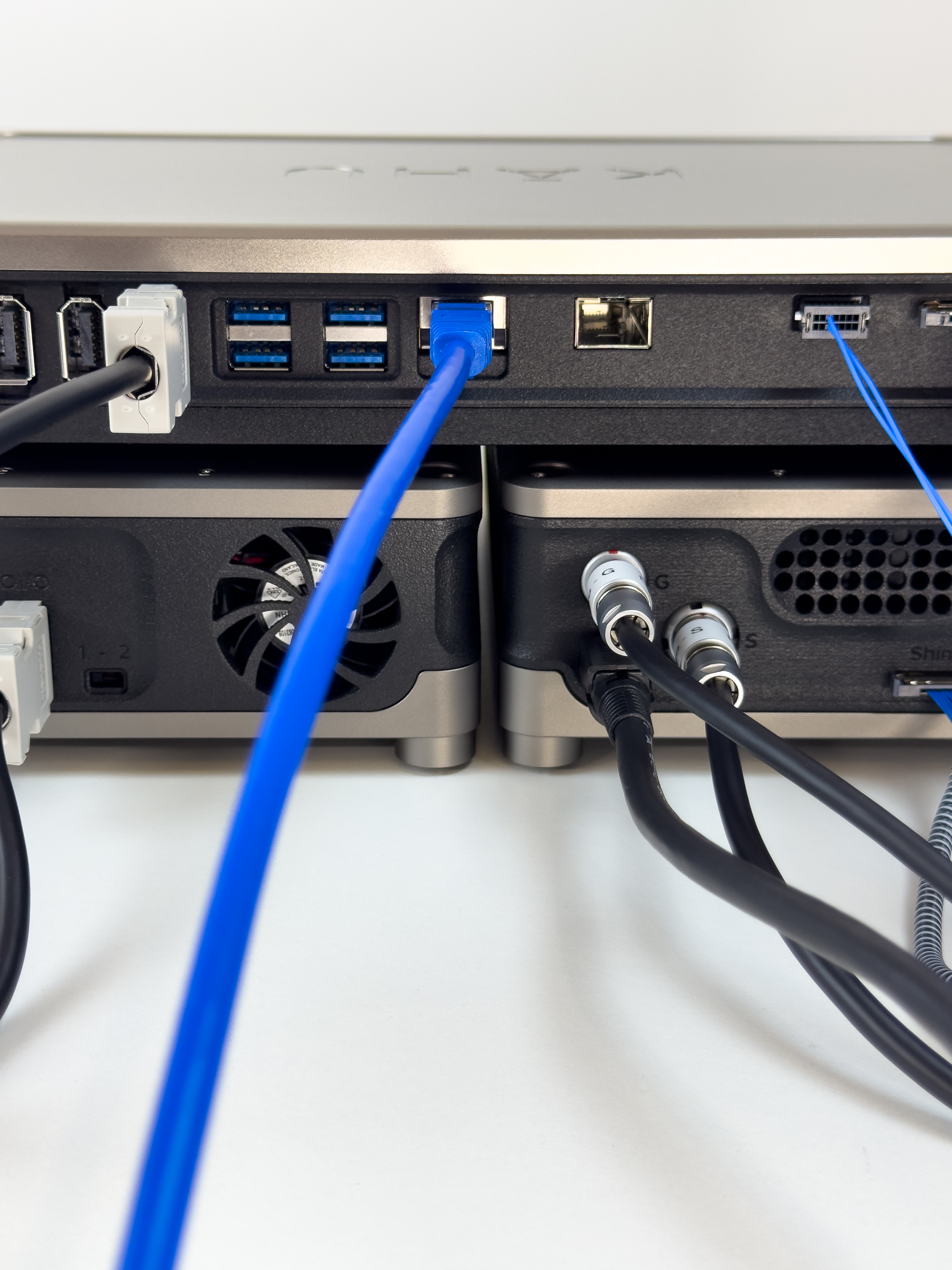
Connect the PT100 and Heater to the Drive Module.

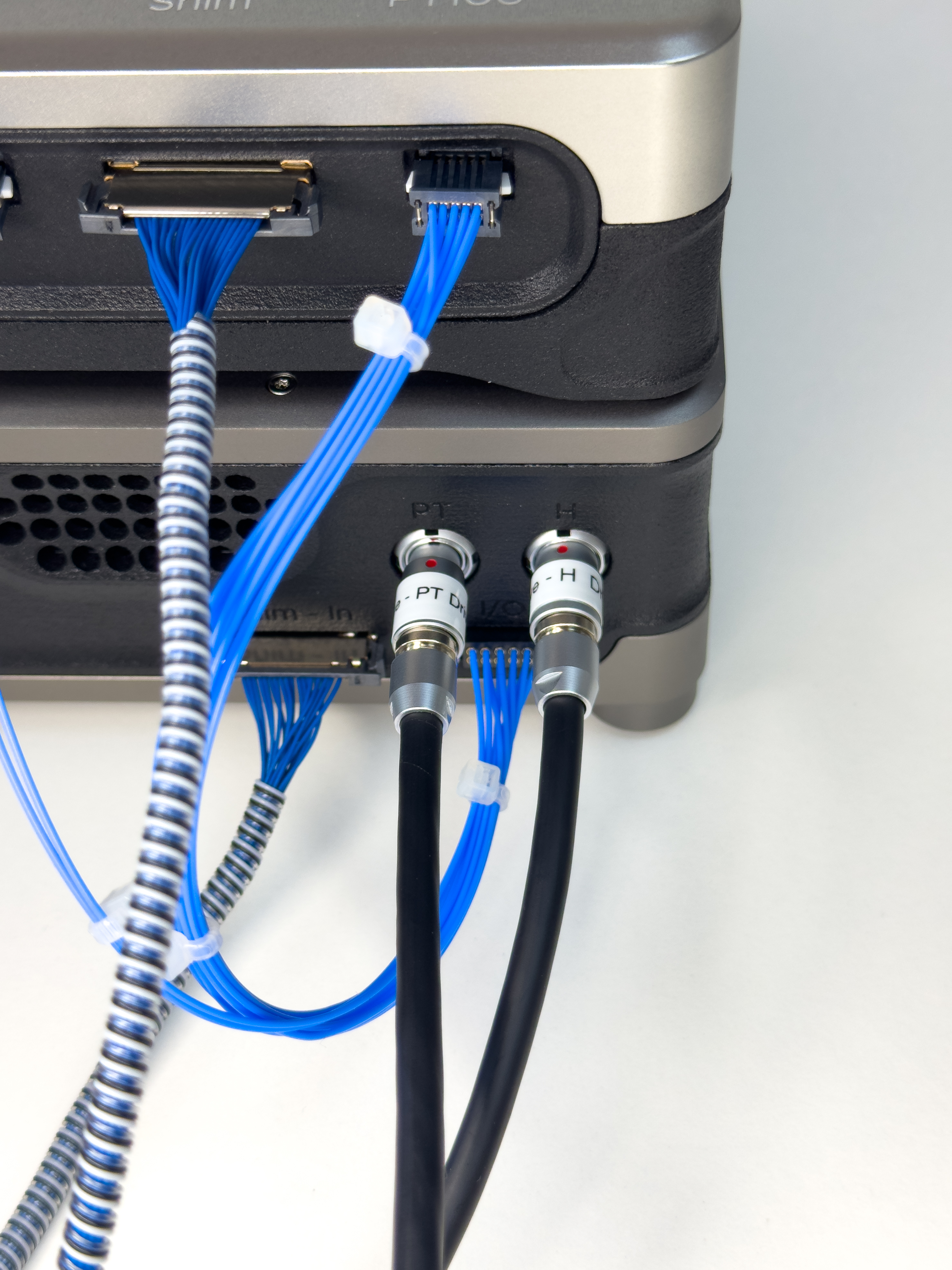
Connect the Gradient and Shim to the Drive Module.

Connect the 3x 24V DC power supplies and the Ethernet cable to Kāhu. Kāhu can either be connected directly to your PC or to a router. See the Software Setup section for more details.

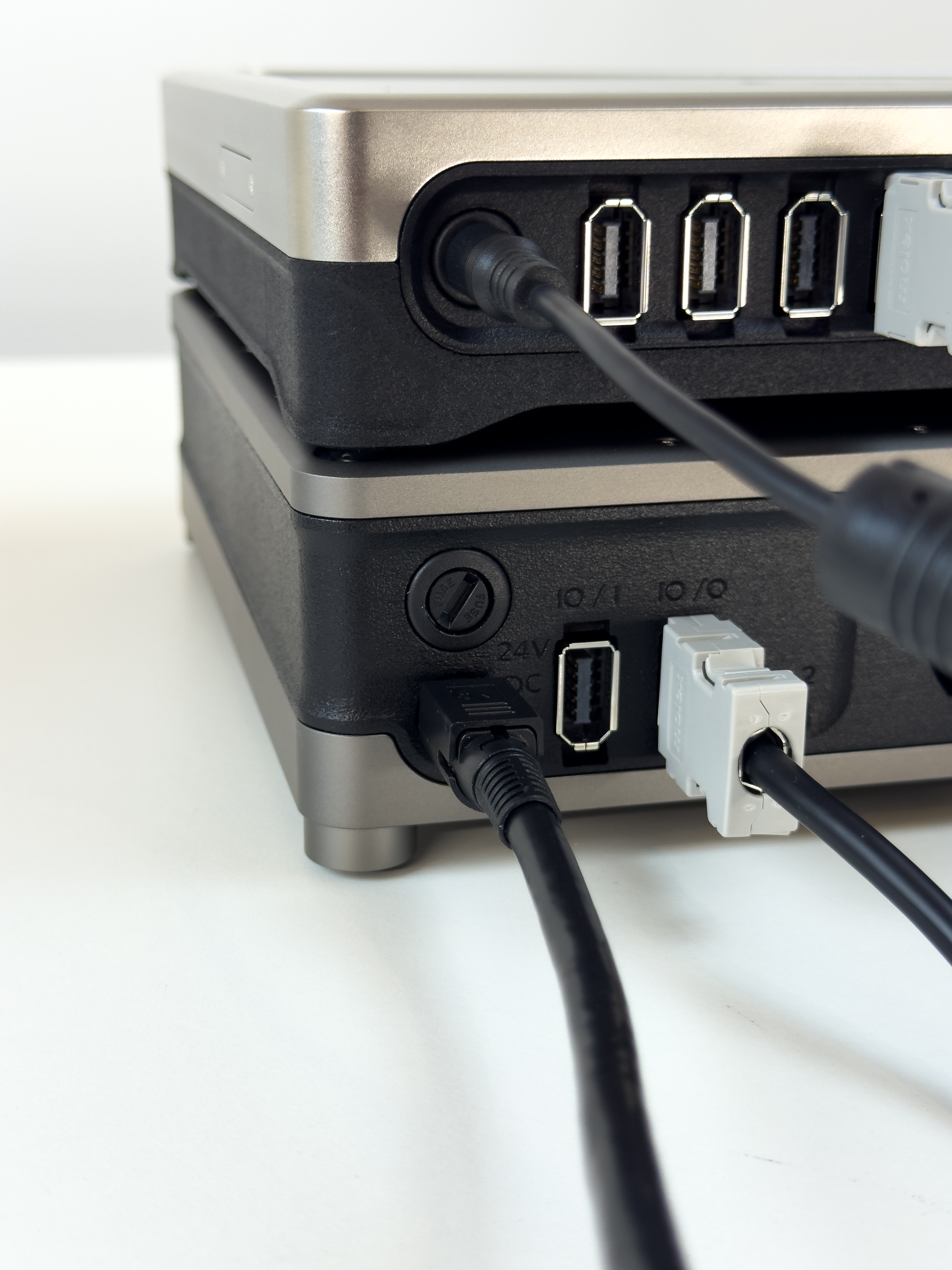
All the necessary Rear cable connections have now been made.

Step 2 - Front cable connections

Begin by connecting the gradient control cables to Kāhu as shown.

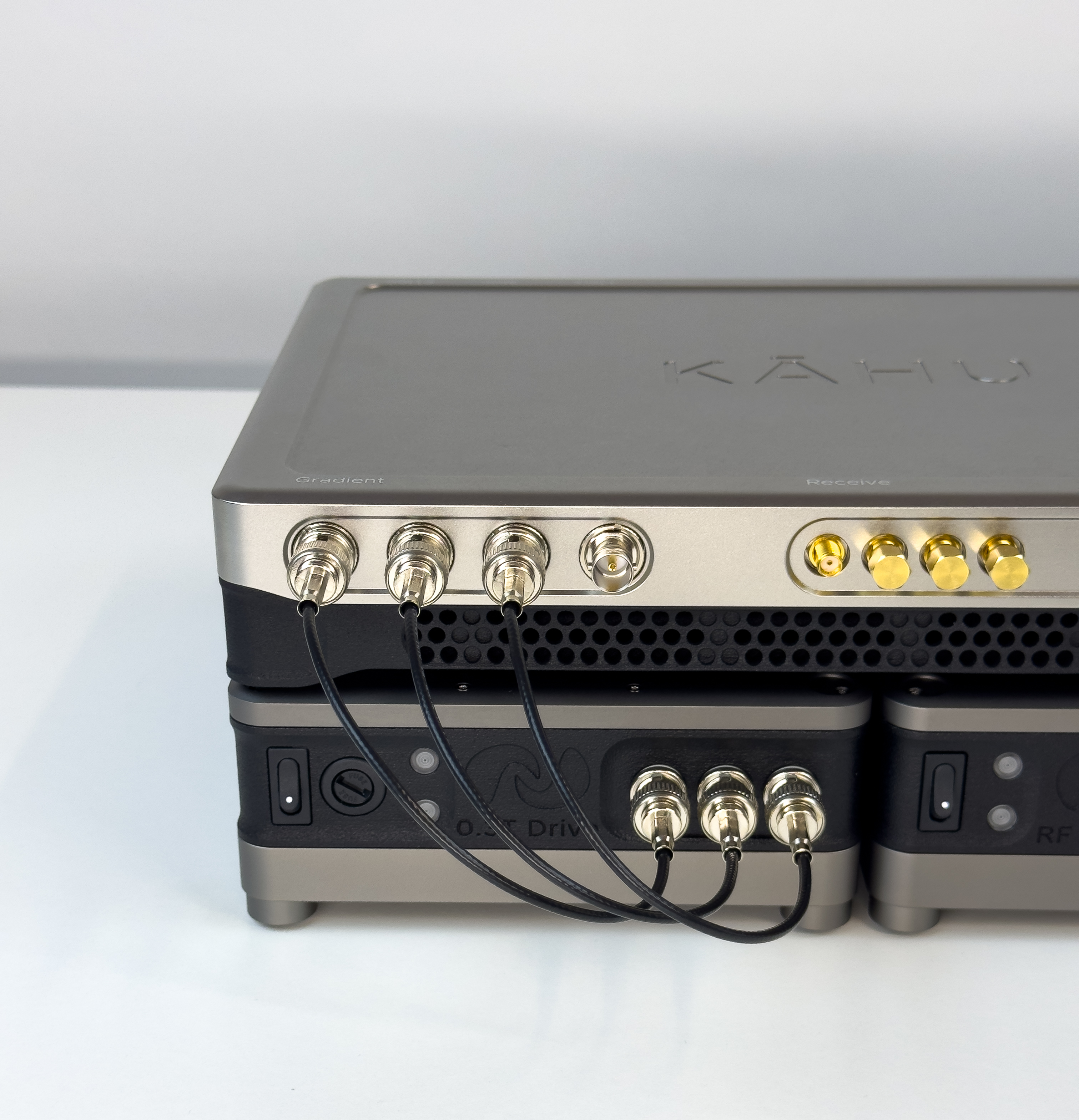
Connect Kahu Rx Channel 0 and Tx Channel 0 to the RF Amplifier.

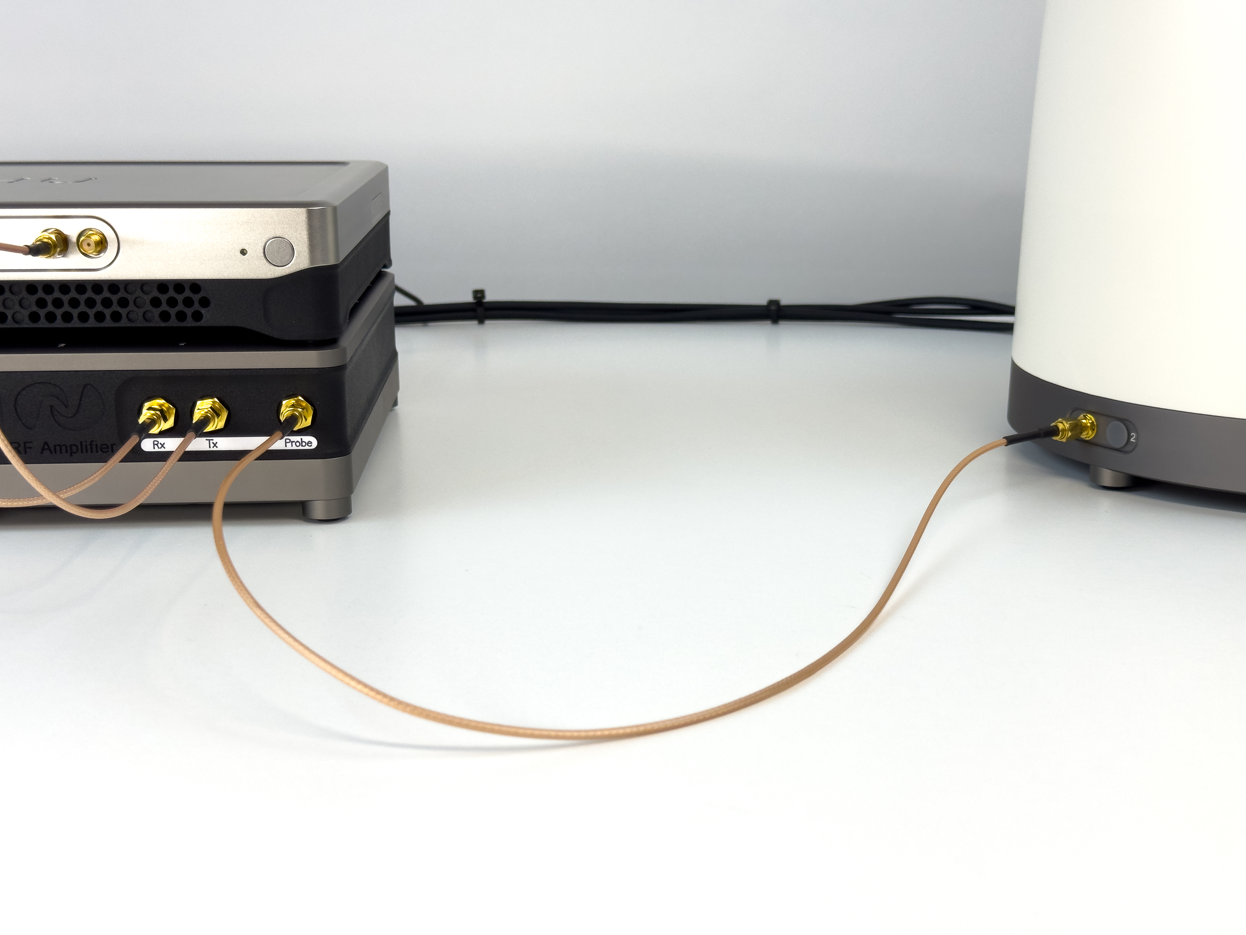
Finish with connecting the Probe to the magnet.

Following this, the Kahu Spectrometer can be powered up.

Attention

Before powering up the Drive and RF amplifier modules, ensure that Kāhu has finished powering up by connecting to it. See the next section for details on how to connect to Kāhu. Similarly, before shutting down Kāhu, ensure Drive and RF amplifier modules are turned off.

The Drive and RF amplifier module can now be powered up.

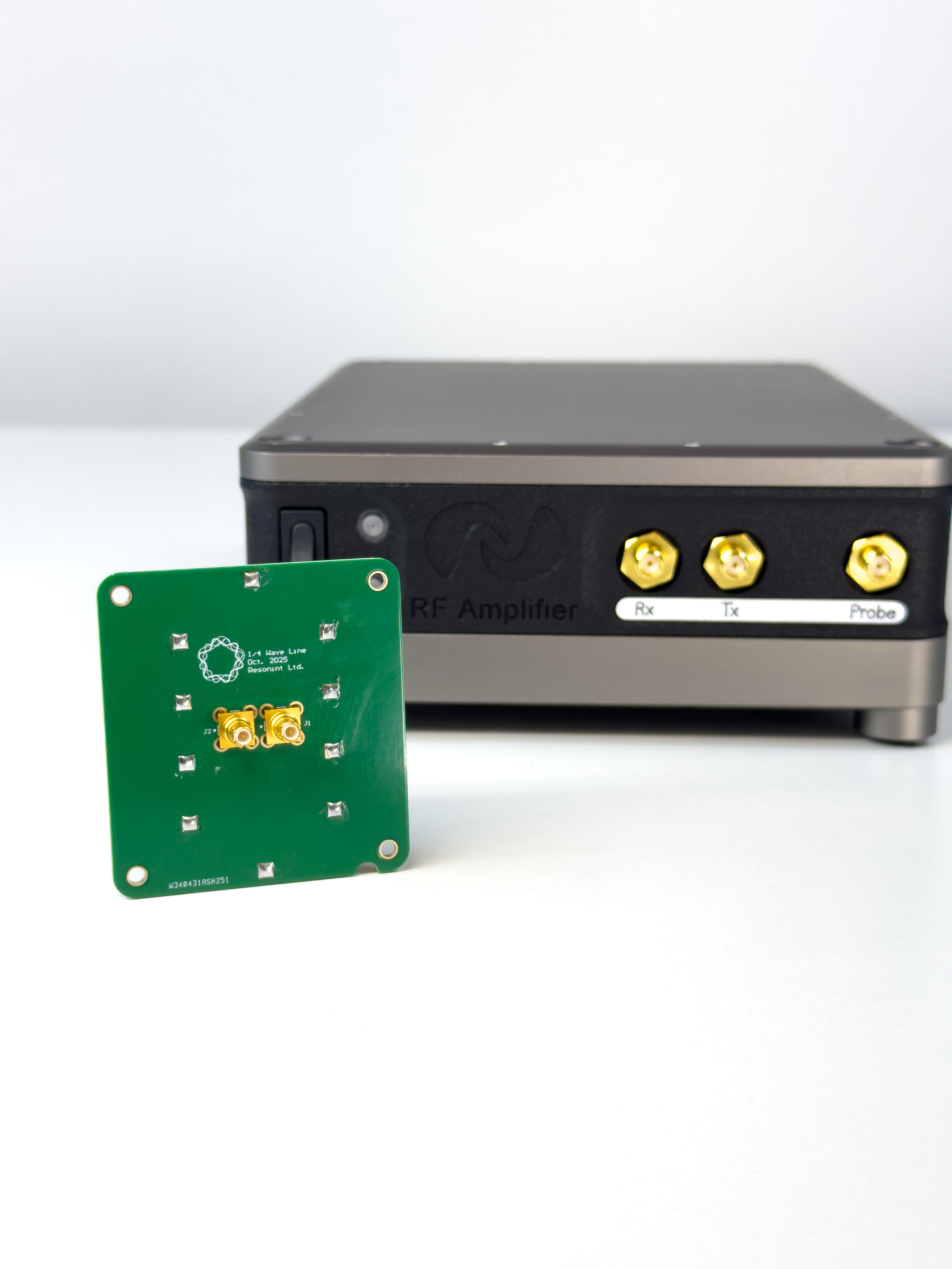
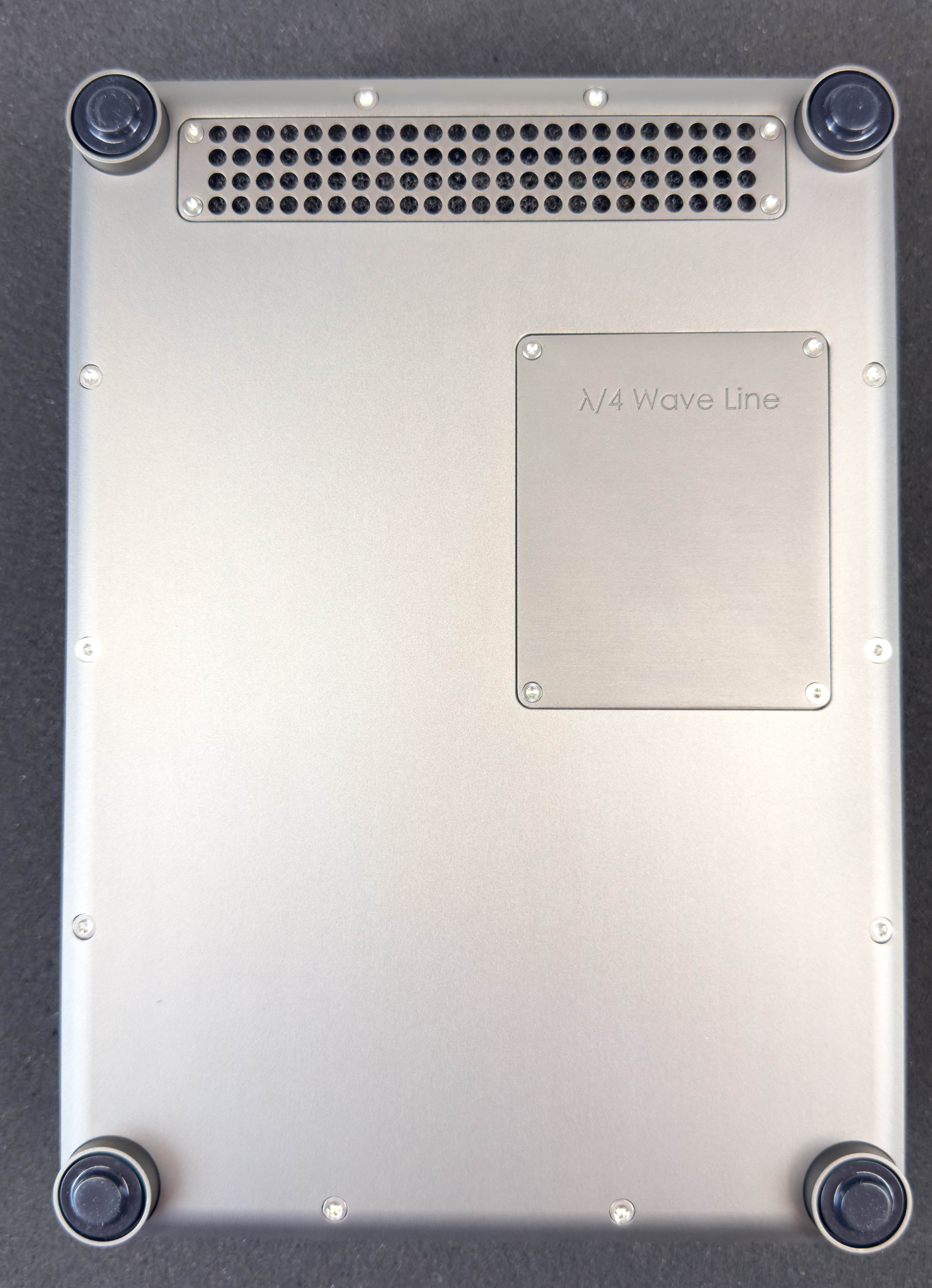
How to retune the RF Amplifier

The 5W RF Amplifier module can be retuned by swapping the 1/4 Wave Line module.

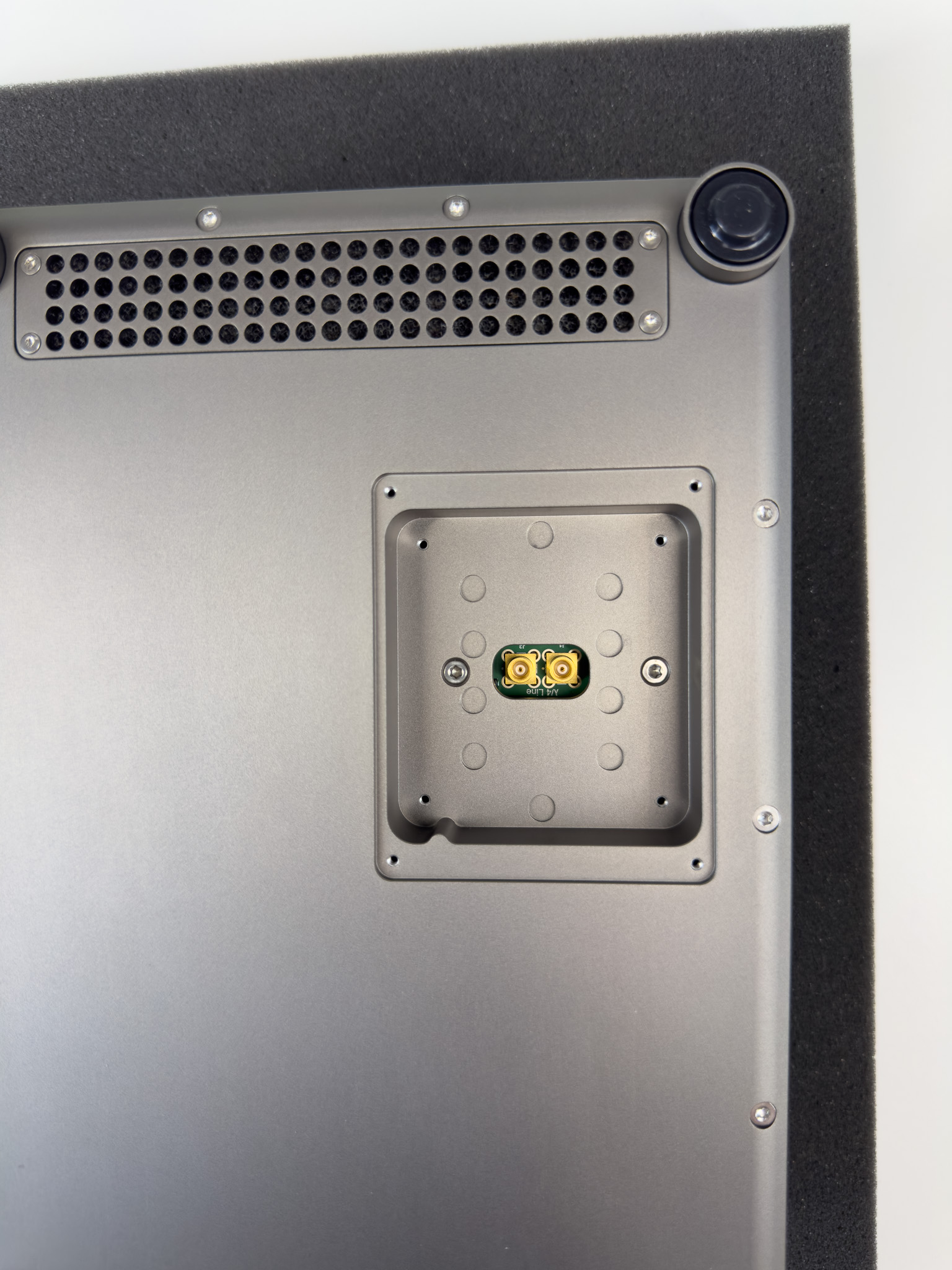
Remove the 4 screws on the 1/4 Wave panel. You can find this on the underside of the Amplifier.

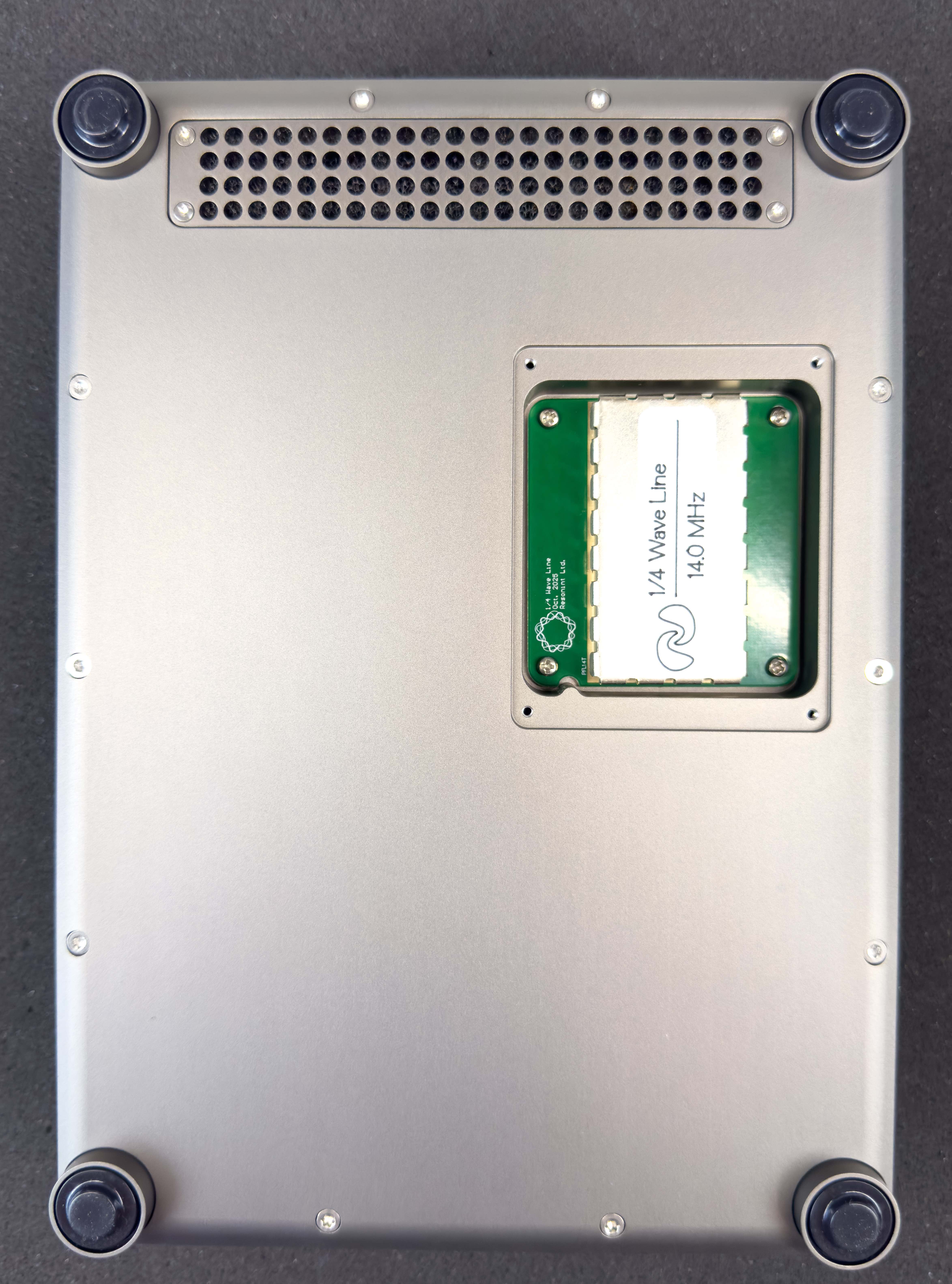
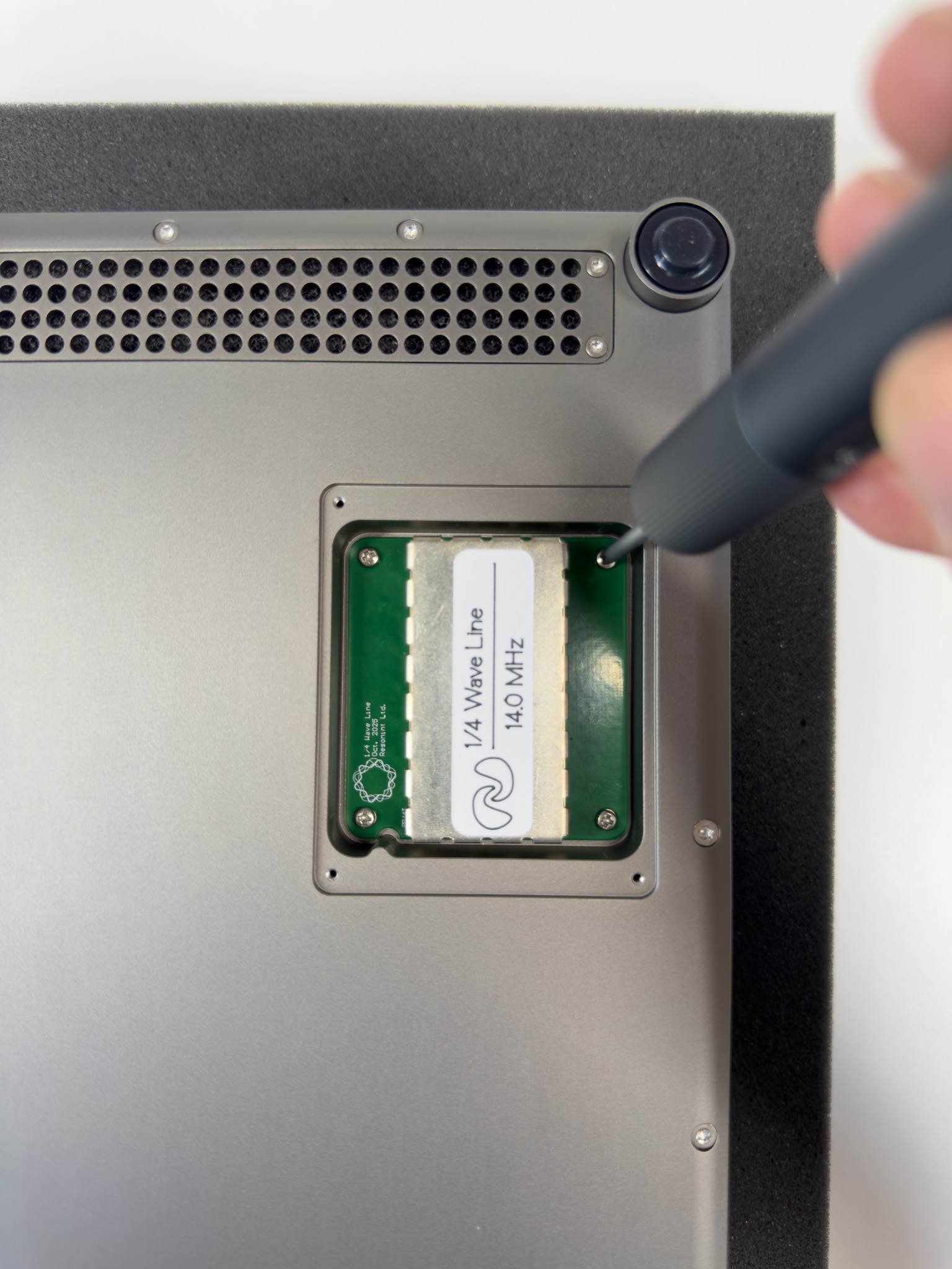
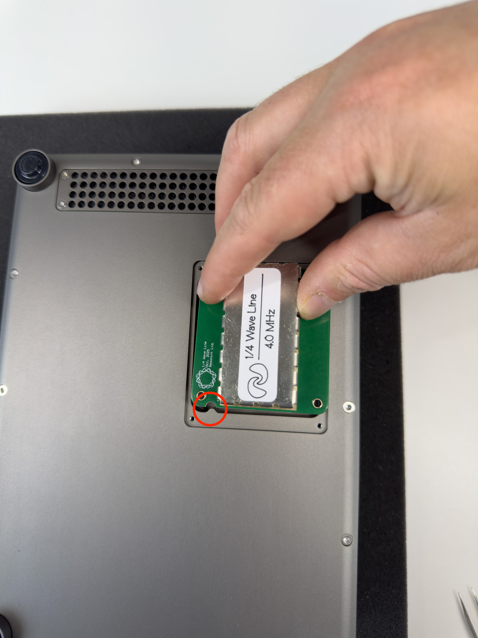
Remove the 4 phillips screws from the 1/4 wave module and carefully pull the module out to disconnect it from the amplifier.

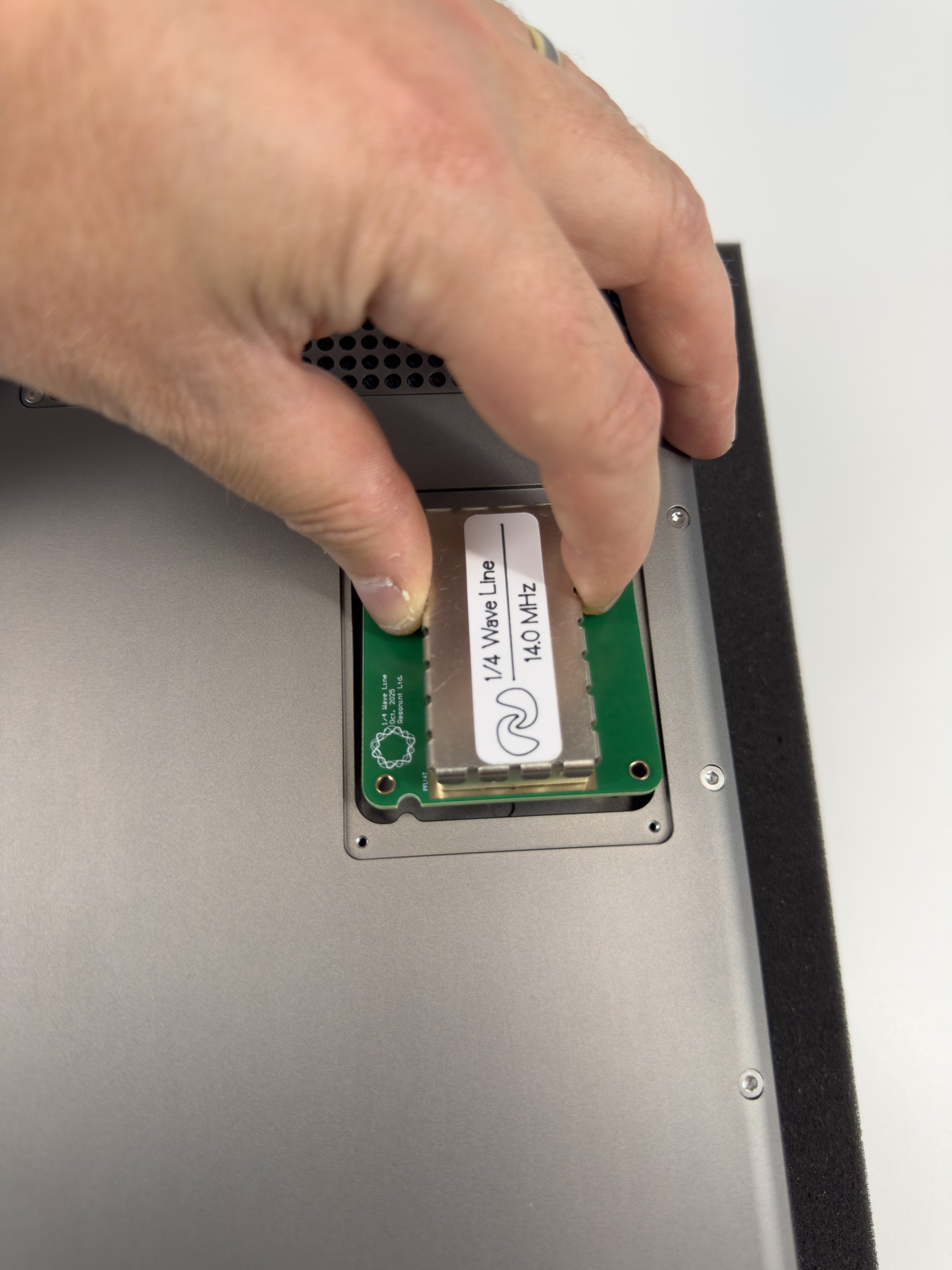
Insert the replacement 1/4 wave module, taking care to align the notch correctly. Press to click it into place and fasten to secure. Finish by refitting the 1/4 Wave panel.

Software Setup

Installing KāhuLab

1. Insert the provided USB drive into your PC or laptop and navigate to it in your file browser.

2. Double click KahuLab-Setup.exe and follow the install process.

3. Once the install is complete, tick the Run KahuLab box and click Finish. KāhuLab is customized version of JupyterLab Desktop. When the application opens you will see the name “jupyterlab”.

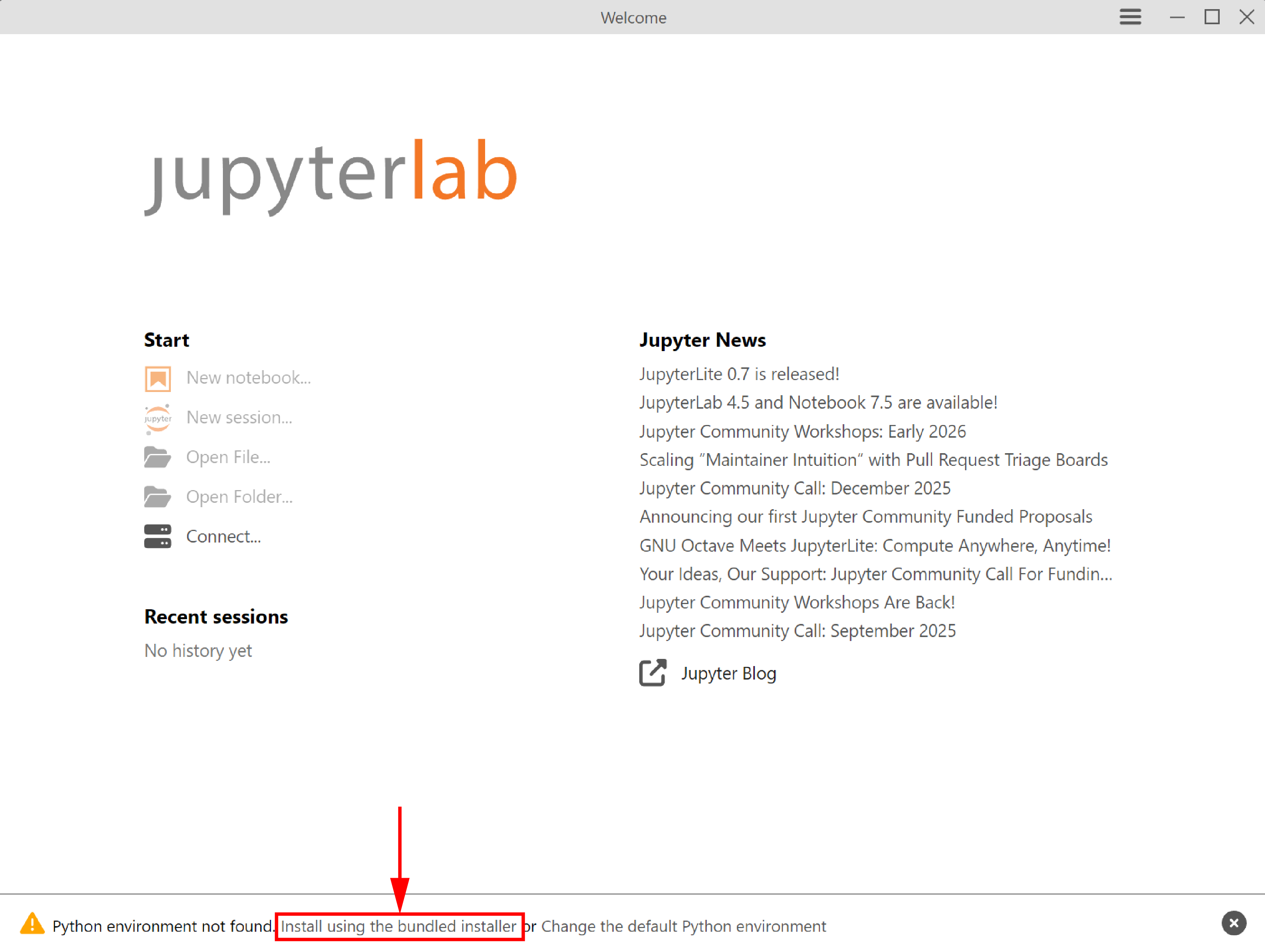
4. Once KāhuLab opens you will see an alert displayed at the bottom of the app that says “Python environment not found.”

Installing the default python environment

5. Click “Install using the bundled installer”.

6. Open your file browser and copy the kahu-workspace.zip file onto your PC or laptop.

7. Right click the copy of the file and select Extract All.

8. Return to KāhuLab.

9. Once the python environment is installed, the Open File and Open Folder buttons will be activated.

10. Close and re-open KāhuLab using the desktop shortcut or start menu.

11. Click Open Folder and navigate to where you extracted the kahu-workspace folder from the zip file. Select this folder and click Open.

12. The KāhuLab interface will now load.

13. Double click the file install.ipynb on the left and when it has loaded, click Run > Run All Cells to install matipo-python library and set up the default configuration.

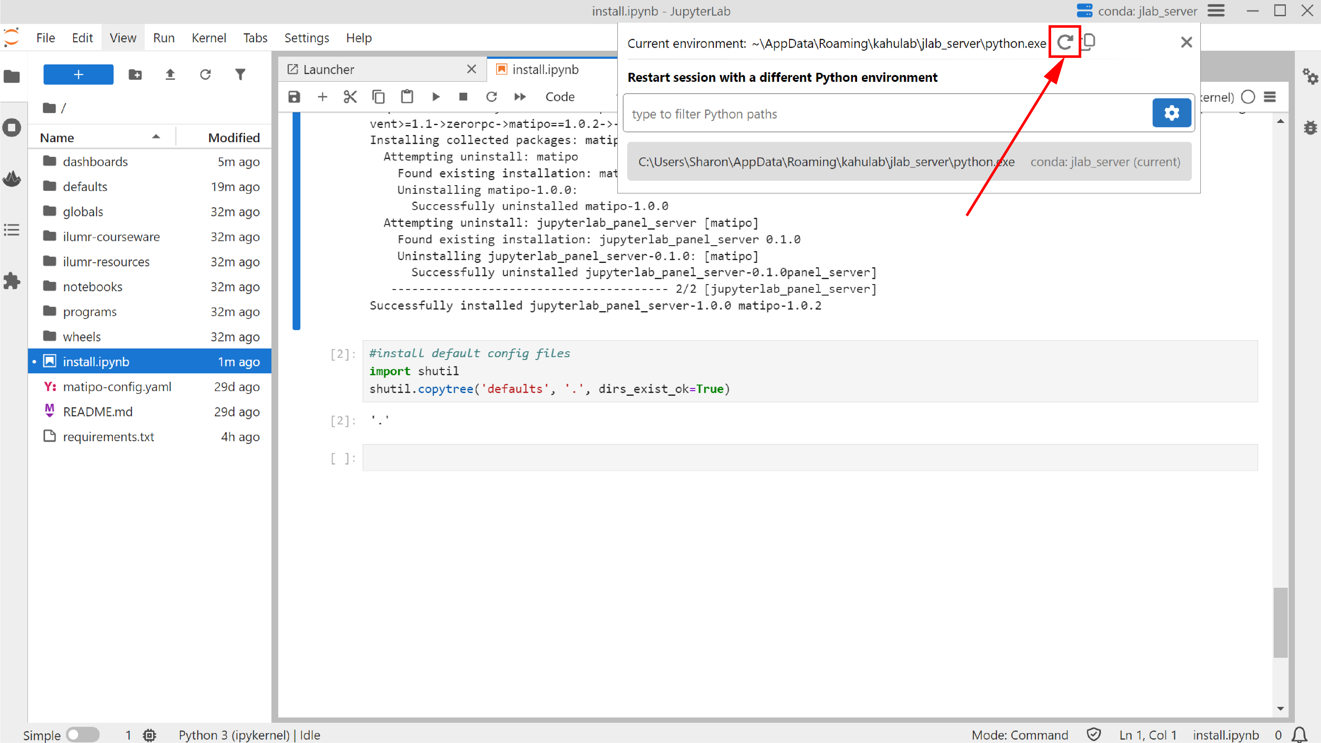
14. Click “conda: jlab_server” in the top menu bar.

Restarting the session

15. Click the reload icon to restart the session.

Connecting to Kāhu

When connecting to Kāhu by direct ethernet cable from a PC, assign a manual IP with settings:

Address: 192.168.137.1 Netmask: 255.255.255.0 Gateway: 192.168.137.1

Kāhu may also be connected to a router via ethernet cable. In this case check the router admin page for the automatically assigned IP address. This IP address must be set in matipo-config.yaml file located in the kahu-workspace folder as the device_address.

After saving matipo-config.yaml you will need to click “conda: jlab_server” in the top menu bar then click the reload icon to restart the session.

The default matipo-config.yaml file is created when you run install.ipynb, and contains the default Kāhu device_address: 192.168.137.2

Trouble Shooting

If you see the error similar to the following when loading a dashboard:

Error: [Errno 2] No such file or directory: 'C:\\Users\\user\\programs/find_freq.py'; in file C:\Users\user\Documents\kahu-workspace\dashboards\Utilities.py

You have not created the matipo-config.yaml file and need to complete steps 13-15 in the Installing JupyterLab section.

System Calibration

Click the icon on the left to open the launcher. There will be two categories: General and ilumr which may be collapsed, expanded, and repositioned.

To check the connection open the System dashboard. If the connection is successful, it will load and display the magnet temperature plot. If it is unable to connect it will print a timeout error.

Wait until the temperature has stabilised to 30℃ before continuing with the calibration setup.

Noise Check

Once the system temperature is stable, you can perform a Noise Check. This dashboard allows you to assess whether the operating environment is suitable for Kāhu with no large sources of electrical interference. When you run this dashbaord the system will measure and display the environmental noise level.

Click “Run” for a single measurement or “Run Loop” for continuous measurements.

Interference will show up as large spikes extending higher then the baseline noise level. The RMS of the noise signal is displayed in the top left, and should be less than 0.3 µV when using a dwell time of 1 µs.

Note

Note that the data shown here is raw data from the hardware decimator, which does not have a flat frequency response, so the noise spectrum (right-hand plot) will normally have a bell-curve-like shape as shown below.

Find Frequency

The next dashboard to run is Find Frequency which uses an free induction decay (FID) pulse sequence with several dwell time increments in order to determine the NMR frequency of the magnet.

Begin by setting up the sample grip with a collar and shim sample as shown.

Center the provided shim sample with the window in the depth gauge and then insert into the magnet.

Press “Run” to perform the experiment and determine the NMR frequency. The new frequency value is automatically saved and can be found in the following location:

globals/frequency.yaml

Tune Match

The RF probes supplied with Kāhu have been tuned to the magnet’s resonant frequency. However, due to differences in operating environments, this frequency may shift slightly. It is important to have the probe tuned to the current magnet frequency, so before running NMR experiments use the Wobble dashboard to check and adjust the probe tuning if required.

In the graph below, the dotted line indicates the magnet frequency, taken from the frequency found in the previous dashboard. This is an example of a well tuned probe, small offsets from the NMR frequency are not a problem and may also be caused by a change in sample. Try removing the shim sample while running the wobble in looped mode to see the effect.

A well tuned probe should meet the following requirements:

Tune: NMR frequency +/- 0.02MHz

Match: less then 20 µV (20e-6) at NMR frequency

If the probe tunings falls outside of these requirements then please follow the next steps:

1. Click “Run Loop” on the Wobble dashboard.

2. Remove the top disk by rotating anti-clockwise

3. Identify the tune and match capacitors using the provided image. The bottom tune/match capacitor is for coarse adjustment and the top for fine adjustment.

4. Identify the alignment arrows and notches on the capacitors. Each capacitor has a tiny arrow on the turning part and a notch on the rim. One end of the adjustment range is reached when the arrow is aligned with the notch, and the other end is reached when the arrow is pointing in the opposite direction.

5. Use the supplied trimmer too to adjust the fine capacitors to 90° from the notch (the halfway point of its range).

6. Adjust the coarse capacitors to get the tune/match roughly correct.

7. Then use the fine capacitors to refine the tune/match.

Note

Note that the presence of the trimmer tool will shift the value so remove after each small adjustment to check.

Pulse Calibration

Once the tuning/matching of the probe has been confirmed, the pulse power of 90 and 180 degree RF pulses can be calibrated using the Pulse Calibration dashboard.

The default settings should be adequate when using the 11 mm RF probe (provided as default with Kāhu), but the 15 mm RF probe will require a longer Pulse Width (recommended 60 us) and a greater Number of Steps (recommended 100) to achieve a 180 degree tipping angle.

Once pulse calibration is complete, vertical dotted lines will show the amplitudes of the 90 and 180 degree pulses and the settings will be automatically save to the following files (when not calibrating a soft pulse):

• globals/hardpulse_90.yaml

• globals/hardpulse_180.yaml

To calibrate soft pulses for MRI slice experiments, check the Soft Pulse option and set the desired Slice Width. The pulse width will auto-populate with a value that should be suitable. When calibration is finished, the settings will be saved to files named:

• globals/softpulse_90_<slice width>mm.yaml

• globals/softpulse_180_<slice width>mm.yaml

If the 180 degree tipping angle is not reached, the corresponding file will not be created.

Autoshim

The final setup step is determining the electrical shim settings, which is done by Autoshim. The first time this is run after power up (and leaving for some time for the temperature to stabilise) the Coarse setting should be selected in the bottom left for it to start from scratch. A Quick shim can be run periodically to re-optimise the homogeneity if it has drifted (due to small changing thermal gradients in the magnet). The shim values are automatically saved to the shims file (with values in the range [-1, 1]):

globals/shims.yaml

Conclusion

With calibration complete, you can proceed to run the other dashboard apps, e.g. 2D RARE, or notebooks. Example notebooks have been included in the ilumr-resources/notebooks directory of the workspace, and educational labs in the ilumr-courseware directory.